5 Data wrangling I: dplyr verbs
Getting started
Download the “data_wrangling_notes.Rmd” and “model_quality_notes.Rmd” documents from Canvas and open in RStudio.
Open the group solutions document. This is where we’ll track our notes.
Check to see whether you have the
boot,caret, andgridExtrapackages installed:If not, then install them from the console. For example:
Today’s plan:
- Discuss yesterday’s homework & tie up any loose ends
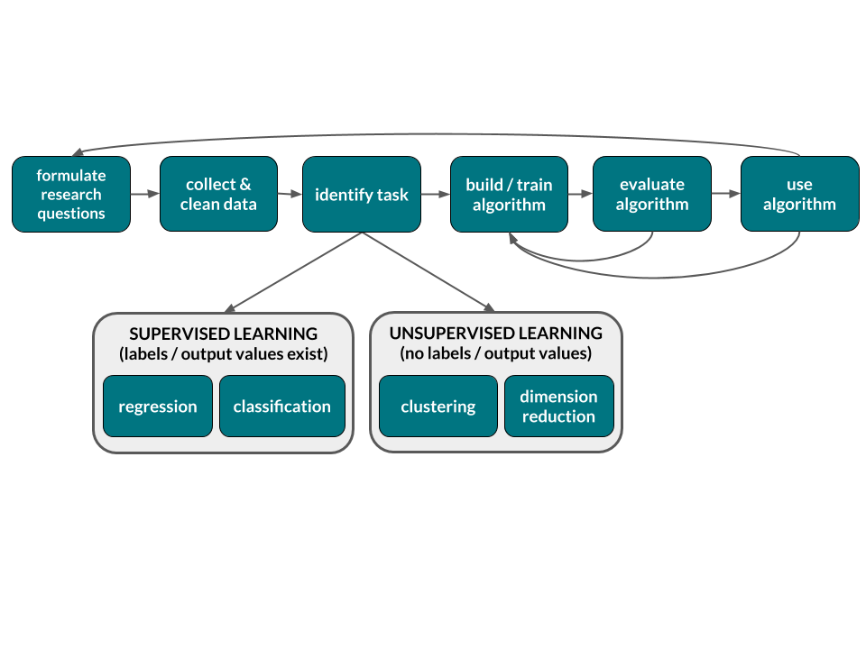
- Explore two more important steps of the machine learning workflow:
- Data wrangling
- Evaluating model quality
5.1 dplyr verbs
Though models and algorithms often get all the glory in the fields of machine learning / statistics / data science, data wrangling is as or more important. We can know all the theory in the world, but if we don’t have facility in working with data, we won’t get anywhere. Today we’ll explore how to wrangle tidy data2 using the dplyr package (which is part of the broader tidyverse which includes ggplot2). In the dplyr grammar, there are 6 main data transformation verbs (actions):
| verb | action | example |
|---|---|---|
select() |
take a subset of columns | select(x, y), select(-x) |
mutate() |
create a new variable, ie. column | mutate(x = ___, y = ___) |
arrange() |
reorder the rows | arrange(x), arrange(desc(x)) |
filter() |
take a subset of rows | filter(x == __, y > __) |
summarize() |
calculate a numerical summary of a variable | summarize(mean(x), median(y)) |
group_by() |
group the rows by a specified column | group_by(x) %>% summarize(mean(y)) |
We can apply one or more verbs through a series of pipes (%>%):
# Apply 1 verb to my_data
my_data %>%
  verb_1(___)

# Apply 2 verbs to my_data
my_data %>%
  verb_1(___) %>%
  verb_2(___)
5.2 Exercises
The fivethirtyeight article
The Ultimate Halloween Candy Power Ranking analyzed data produced from this experiment which presented subjects with a series of head-to-head candy match-ups and asked them to indicate which candy they preferred. You can load these data from the fivethirtyeight package:
# Load data
library(fivethirtyeight)
data("candy_rankings")

# Examine the codebook
?candy_rankings

# Store under a shorter name
candy <- candy_rankings
We’ll wrangle these data below. In each exercise, first identify which dplyr verbs will be useful.
Sort the candies
Find the candies
- Define new variables
Create a new data set,candy_newwith the following new variables:- Redefine
sugarpercentfrom 0-1 scale to the 0-100 scale - Define a
choc_peanutvariable which identifies candies that contain both chocolate & peanuts/almonds
- Redefine
Calculate some stats
Pipe series
Each column is a variable and each row is a case. See Wickham, Tidy Data and Wickham and Grolemund, Tidy Data for more.↩︎