11 Homework 1: Visualizing & modeling relationships

Directions:

Start a new RMarkdown document.
Load the following packages at the top of your Rmd: dplyr, ggplot2, fivethirtyeight
When interpreting visualizations, models, etc, be sure to do so in a contextually meaningful way.
This homework is a resource for you. Record all work that is useful for your current learning & future reference. Further, try your best, but don’t stay up all night trying to finish all of the exercises! We’ll discuss any questions / material you didn’t get to tomorrow.
Solutions are provided at the bottom. You are all experienced learners and so know that you’ll get more out of this homework if you don’t peak at the solutions unless and until you really, really, really need to.

Goals:

The goal of this homework is to get extra practice with visualizing relationships, constructing models, and interpreting models. You’ll also explore three new ideas:

interactions between predictors
controlling for covariates
residuals & least squares estimation

11.1 Interaction

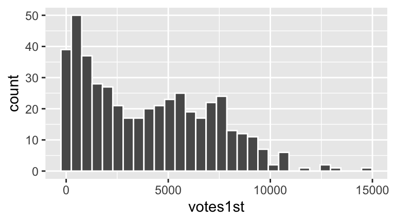
In their research into the “campaign value of incumbency,” Benoit and Marsh (2008) collected data on the campaign spending of 464 candidates for the 2002 elections to the Irish Dail. The authors provide the following data set

campaigns <- read.csv("https://www.macalester.edu/~ajohns24/data/CampaignSpending.csv") %>% 
  select(votes1st, incumb, totalexp) %>% 
  na.omit()

which, for all 464 candidates, measures many variables including

variable	meaning
`votes1st`	number of “1st preference” votes the candidate received
`incumb`	`No` if the candidate was a challenger, `Yes` if the candidate was an incumbent
`totalexp`	number of Euros spent by the candidate’s campaign

The votes received varies by candidate. Our goal is to explain some of this variability:

ggplot(campaigns, aes(x = votes1st)) + 
    geom_histogram(color = "white")

Warm-Up: Votes vs Incumbency
We might be able to explain some of the variability in votes received by a candidate’s incumbency status.
1. Construct a visualization of the relationship between votes1st and incumb.
2. Construct a model of votes1st by incumb, write out the model formula, & interpret all coefficients.
3. From the model coefficients, compute the average votes received by incumbents and the average votes received by challengers. We’ll learn another method to do these computations tomorrow.

Warm-Up: Votes vs Incumbency Status & Campaign spending
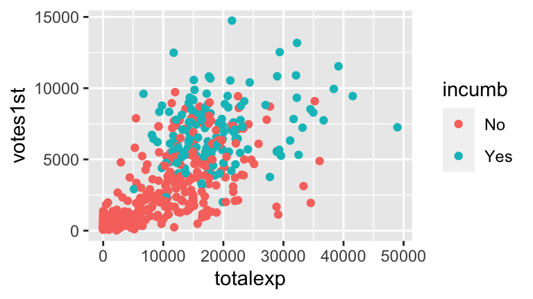
Let’s incorporate campaign spending into our analysis.
1. Construct 1 visualization of the relationship of votes1st vs incumb and totalexp.
2. Construct a model of votes1st by incumb and totalexp. Store this as model2. Write out the following formulas:
  - the full model formula
  - a simplified formula for challengers
  - a simplified formula for incumbents
3. Interpret all coefficients. Remember: your interpretation of the incumb coefficient here should be different than in the first model since the models contain different sets of predictors.
4. Use this model to predict the number of votes received by the following candidates.
  - Candidate 1: a challenger that spends 10,000 Euros
  - Candidate 2: an incumbent that spends 10,000 Euros
5. Check your predictions using the predict() function.

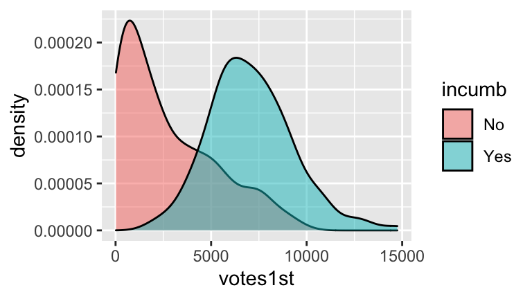
Check out a plot of model2. (RStudio code is included FYI, but don’t worry about it for now!)
```
ggplot(campaigns, aes(x = totalexp, y = votes1st, color = incumb)) + 
  geom_point(size = 0.5) + 
  geom_line(aes(y = model2$fitted.values))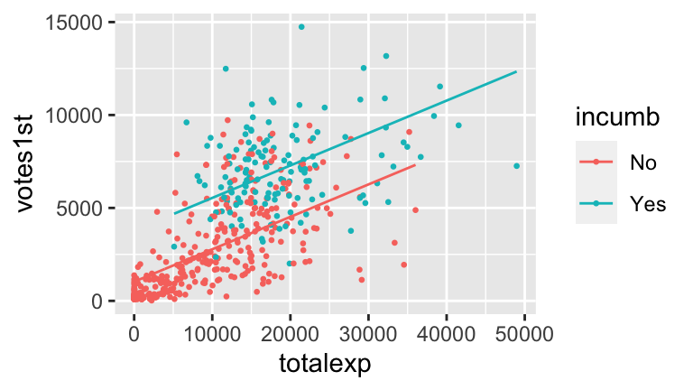
```
Since the lines are parallel, this model assumes that incumbents and challengers enjoy the same return on campaign spending. However, notice from the plot that this may not be the best assumption. Rather, without the parallel model constraint, the trend looks more like this (you’ll make this plot later):
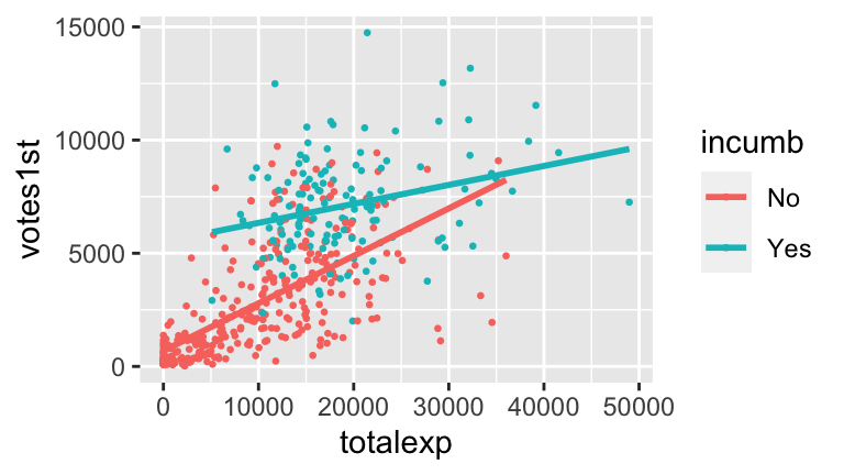To allow our models for challengers and incumbents to have different intercepts and different slopes, we can type totalexp * incumb instead of totalexp + incumb in the lm function:
```
new_model <- lm(votes1st ~ totalexp * incumb, campaigns)
summary(new_model)
```
1. The totalexp:incumbYes term that you see in the model summary is called an interaction term. Mathematically, it’s the product of these two variables, totalexp * incumbYes. With this in mind, write down the model formulas:
  - the full model formula (of the form votes1st = a + b totalexp + c incumbYes + d totalexp * incumbYes)
  - a simplified formula for challengers (of the form votes1st = a + b totalexp)
  - a simplified formula for incumbents (of the form votes1st = a + b totalexp)
2. Use this model to predict the number of votes received by the following candidates. Calculate these by hand & then check your work using predict().
  - Candidate 1: a challenger that spends 10,000 Euros
  - Candidate 2: an incumbent that spends 10,000 Euros
3. You can visualize this model by adding a geom_smooth() to your scatterplot:
```
ggplot(campaigns, aes(x = totalexp, y = votes1st, col = incumb)) + 
    geom_point() + 
    geom_smooth(method = "lm")
```
  You should notice the interaction between campaign spending & incumbency status, i.e. that the relationship between votes & spending differs for incumbents and challengers. With this in mind, comment on what the differing intercepts and differing slopes indicate about the relationship between the three variables of interest.
4. Putting this all together, interpret all four model coefficients from new_model. Hint: As we have for models in the past, look back to the equations for the incumbent & challenger models.

Interaction

In modeling $y$, predictors $x_1$ and $x_2$ interact if the relationship between $x_1$ and $y$ differs for different values of $x_2$.

11.2 Covariates

In examining multivariate models, we’ve seen that adding explanatory variables to the model helps to better explain variability in the response. For example, compare the plot on the left which ignores the grouping variable vs the plot on the right that includes it:

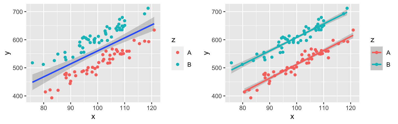
However, explaining variability isn’t the only reason to include multiple predictors in a model. When exploring the relationship between response $y$ and predictor $x_1$, there are typically covariates for which we want to control. For example, in comparing the effectiveness of 2 drug treatments, we might want to control for patients’ ages, health statuses, etc.

We’ll explore the concept of controlling for covariates using the CPS_2018 data. These data, obtained through the Current Population Survey, contains labor force characteristics for a sample of workers in 2018. We’ll look only at 18-34 year olds that make under $250,000 per year:

cps <- read.csv("https://www.macalester.edu/~ajohns24/data/CPS_2018.csv") 

cps <- cps %>% 
    filter(age >= 18, age <= 34) %>% 
    filter(wage < 250000)

head(cps, 3)
##    wage age education    sex marital   industry    health hours citizenship
## 1 75000  33        16 female  single management      fair    40         yes
## 2 33000  19        16 female  single management very_good    40         yes
## 3 43000  33        16   male married management      good    40         yes
##   disability education_level
## 1         no       bachelors
## 2         no       bachelors
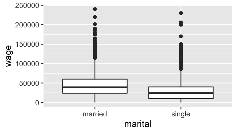
## 3         no       bachelors

We’ll use these data to explore the pay gap between married and single workers, illustrated and modeled below:

ggplot(cps, aes(y = wage, x = marital)) + 
  geom_boxplot()

cps_mod1 <- lm(wage ~ marital, data = cps)
summary(cps_mod1)
## 
## Call:
## lm(formula = wage ~ marital, data = cps)
## 
## Residuals:
##    Min     1Q Median     3Q    Max 
## -46145 -20093  -6145  11855 200907 
## 
## Coefficients:
##               Estimate Std. Error t value Pr(>|t|)    
## (Intercept)    46145.2      921.1   50.10   <2e-16 ***
## maritalsingle -17052.4     1127.2  -15.13   <2e-16 ***
## ---
## Signif. codes:  0 '***' 0.001 '**' 0.01 '*' 0.05 '.' 0.1 ' ' 1
## 
## Residual standard error: 29890 on 3167 degrees of freedom
## Multiple R-squared:  0.0674,	Adjusted R-squared:  0.0671 
## F-statistic: 228.9 on 1 and 3167 DF,  p-value: < 2.2e-16

From the model coefficients we see that: On average, married workers make $46,145.20 per year and single workers make $17,052.40 less per year than married workers.

Correlation does not imply causation
If you’re single, this model probably didn’t inspire you to go out and find a spouse. Why? Just because there’s a relationship between wages and marital status doesn’t mean being single causes a person to earn less. List a few confounding variables that might explain this relationship between wages and marital status.

Including covariates / confounding variables
One variable that might explain the observed relationship between wages & marital status is age - older people both tend to make more money and are more likely to be married. We can control for this covariate by including it in our model.
1. Fit and summarize a model of wage by marital and age that does not include an interaction term.
```
cps_mod2 <- ___
___(cps_mod2)
```
2. Construct a visualization of this relationship that eliminates individual data points but includes the model smooth or trend. Does it appear that age and marital status interact? Explain.
```
___() + 
   ___()
```
3. Compare two workers that are both 20 years old, but one is married and the other is single. By how much do their predicted wages to differ? Use the model formula to calculate this difference and the plot to provide intuition.
4. Compare two workers that are both 30 years old but one is married and the other is single. By how much do their predicted wages to differ?
5. If you’d like extra practice, interpret every coefficient in this model.

Controlling for more covariates
Taking age into account added some insight into the discrepancy between single and married workers’ wages. Let’s see what happens when we control for even more variables. To this end, model a person’s wage by their marital status while controlling for their age, years of education, and the job industry in which they work. For simplicity, eliminate all interaction terms:
```
cps_mod3 <- ___
summary(cps_mod3)
```
1. This is difficult model to visualize since there are 2 quantitative predictors (age and education) and 2 categorical predictors (marital and industry) with a possible 12 category combinations (2 marital statuses * 6 industries). If you had to draw it, what would it look like?
  - 12 parallel lines
  - 12 non-parallel lines
  - 12 parallel planes
  - 12 non-parallel planes
2. Compare two workers that are both 20 years old, have 16 years of education, and work in the service industry. If one is married and the other is single, by how much do their predicted wages to differ?
3. Compare two workers that are both 30 years old, have 12 years of education, and work in the construction industry. If one is married and the other is single, by how much do their predicted wages to differ?
4. In light of b & c, interpret the maritalsingle coefficient.
5. In conclusion, we saw differet maritalsingle coefficients in each of cps_mod1, cps_mod2, and cps_mod3`. Explain the significance of the difference between these measurements - what insight does it provide?

Extra interpretation practice
If you’d like extra practice, answer the following questions related to the coefficients in cps_mod3.
1. What is the reference level of the industry variable?
2. For fixed education, marital status, and age, in what industry do workers make the most money? The least?
3. Interpret the education coefficient.
4. Interpret the industrymanagement coefficient.

11.3 Least Squares Estimation

Thus far you’ve been using RStudio to construct models and have focused on interpreting the output. Now let’s discuss how this first step happens, ie. how sample data are used to estimate population models. Due to their serious cuteness, let’s use some penguin data!

# IN YOUR CONSOLE: install the palmerpenguins package
# DO NOT PUT THIS IN YOUR RMD!!
remotes::install_github("allisonhorst/palmerpenguins")

# IN YOUR RMD: load the package and penguins data
library(palmerpenguins)
data(penguins)

# Keep only the 2 variables of interest
penguins <- penguins %>% 
  select(flipper_length_mm, body_mass_g) %>% 
  na.omit()

# IN YOUR CONSOLE: check out the "codebook"
?penguins

Let response variable $Y$ be the length in mm of a penguin’s flipper and $X$ be their body mass in grams. Then the (population) linear regression model of $Y$ vs $X$ is

\[Y = \beta_0 + \beta_1 X + \varepsilon\]

Note that the $\beta_i$ represent the population coefficients. We can’t measure all penguins, thus don’t know the “true” values of the $\beta_i$. Rather, we can use sample data to estimate the $\beta_i$ by $\hat{\beta}_i$. That is, the sample estimate of the population model trend is

\[Y = \hat{\beta}_0 + \hat{\beta}_1 X\]

In choosing the “best” estimates $\hat{\beta}_i$, we’re looking for the coefficients that best describe the relationship between $Y$ and $X$ among the sample subjects. In the visual below, we can see that the red line does a better job at capturing this relationship than the blue line does:

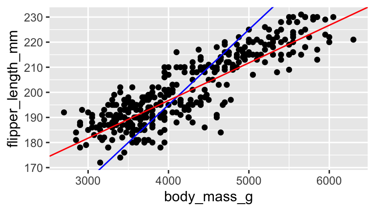
Mainly, on average, the individual points fall closer to the red line than the blue line. The distance between an individual observation and its model value (prediction) is called a residual.

Residuals

Let case $i$ have observed response $Y_i$ and predictor $X_i$. Then the model / predicted value for this case is \[\hat{Y}_i = \hat{\beta}_0 + \hat{\beta}_1 X_i\] The difference between the observed and predicted value is the residual $r_i$: \[r_i = Y_i - \hat{Y}_i\]

We can use our sample data to estimate the population model: \[Y = \hat{\beta}_0 + \hat{\beta}_1 X = 136.73 + 0.015 X\]

penguin_mod <- lm(flipper_length_mm ~ body_mass_g, data = penguins)
summary(penguin_mod)
## 
## Call:
## lm(formula = flipper_length_mm ~ body_mass_g, data = penguins)
## 
## Residuals:
##      Min       1Q   Median       3Q      Max 
## -23.7626  -4.9138   0.9891   5.1166  16.6392 
## 
## Coefficients:
##              Estimate Std. Error t value Pr(>|t|)    
## (Intercept) 1.367e+02  1.997e+00   68.47   <2e-16 ***
## body_mass_g 1.528e-02  4.668e-04   32.72   <2e-16 ***
## ---
## Signif. codes:  0 '***' 0.001 '**' 0.01 '*' 0.05 '.' 0.1 ' ' 1
## 
## Residual standard error: 6.913 on 340 degrees of freedom
## Multiple R-squared:  0.759,	Adjusted R-squared:  0.7583 
## F-statistic:  1071 on 1 and 340 DF,  p-value: < 2.2e-16

Consider the following 2 sample penguins with the following measurements and plotted below. Calculate the residuals (the length of the vertical lines) for both of these penguins.

## # A tibble: 2 x 2
##   flipper_length_mm body_mass_g
##               <int>       <int>
## 1               181        3750
## 2               210        4200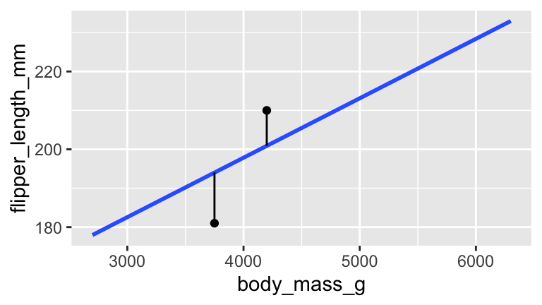

penguin_mod is an lm “object”. Not only does it contain info about the model coefficients, it contains the numerical values of the residuals (residuals) and model predictions (fitted.values) for each penguin in the data set:
```
class(penguin_mod)
## [1] "lm"
names(penguin_mod)
##  [1] "coefficients"  "residuals"     "effects"       "rank"         
##  [5] "fitted.values" "assign"        "qr"            "df.residual"  
##  [9] "xlevels"       "call"          "terms"         "model"
```
1. Create a data frame penguin_results that stores the observed flipper length, model predicted flipper length, and residual for each case in penguins:
```
penguin_results <- data.frame(observed = penguins$flipper_length_mm, 
    predicted = penguin_mod$fitted.values, residual = penguin_mod$residuals)
head(penguin_results, 3)
##   observed predicted   residual
## 1      181  194.0142 -13.014243
## 2      186  194.7780  -8.778039
## 3      195  186.3763   8.623715
```
2. What is the relationship between the observed, predicted, and residual variables in penguin_results? (This shouldn’t be a surprise - it’s just a confirmation of the definition of a residual.)
3. Confirm that, within rounding error, the mean residual equals 0. This property always holds for regression models!
4. Obtain summary statistics of the residuals. Where does this information appear in summary(penguin_mod)?
5. Calculate the standard deviation of the residuals. Where does this information appear in summary(penguin_mod) (within rounding error)? SIDENOTE: The Residual standard error is calculated slightly differently than the standard deviation of residuals. Letting $r_i$ denote a residual for case $i$, $n$ be the sample size, and $k$ being the number of coefficients in our model (here we have 2), then
  \[\text{st dev of residuals} = \frac{\sum_{i=1}^nr_i^2}{n-1} \;\; \text{ and } \;\; \text{Residual standard error} = \frac{\sum_{i=1}^nr_i^2}{n-k}\]

EXTRA: A COMMENT ON THEORY

We hope you learned about linear regression in linear algebra! Suppose we have a sample of $n$ subjects. For subject $i \in \{1,...,n\}$ let $Y_i$ denote the observed response value and $(x_{i1}, x_{i2},...,x_{ik})$ denote the observed values of the $k$ predictors. Then we can collect our observed response values into a vector $y$, our predictor values into a matrix $X$, and our regression coefficients into a vector $\beta$. Note that a column of 1s is included for an intercept term in $X$:

\[ y = \left(\begin{array}{c} y_1 \\ y_2 \\ \vdots \\ y_n \end{array} \right) \;\;\;\; \text{ and } \;\;\;\; X = \left(\begin{array}{ccccc} 1 & x_{11} & x_{12} & \cdots & x_{1k} \\ 1 & x_{21} & x_{22} & \cdots & x_{2k} \\ \vdots & \vdots & \vdots & \cdots & \vdots \\ 1 & x_{n1} & x_{n2} & \cdots & x_{nk} \\ \end{array} \right) \;\;\;\; \text{ and } \;\;\;\; \beta = \left(\begin{array}{c} \beta_1 \\ \beta_2 \\ \vdots \\ \beta_k \end{array} \right)\]

Then we can express the model $y_i = \beta_0 + \beta_1 x_{i1} + \cdots + \beta_k x_{ik}$ for $i \in \{1,...,n\}$ using linear algebra:

\[y = X\beta\] Further, let $\hat{\beta}$ denote the vector of sample estimated $\beta$ and $\hat{y}$ denote the vector of predictions / model values:

\[\hat{y} = X \hat{\beta}\]

Thus the residual vector is

\[y - \hat{y} = X\beta - X\hat{\beta}\] and the sum of squared residuals is

\[(y - \hat{y})^T(y - \hat{y})\]

Challenge: Prove that the following formula for sample coefficients $\hat{\beta}$ are the least squares estimates of $\beta$, ie. they minimize the sum of squared residuals:

\[\hat{\beta} = (X^TX)^{-1}X^Ty\]

11.4 HW1 solutions

Don’t peak until and unless you really, really need to!

#a (one solution)
ggplot(campaigns, aes(x=votes1st, fill=incumb)) + 
    geom_density(alpha=0.5)


#b
model1 <- lm(votes1st ~ incumb, campaigns)
summary(model1)
## 
## Call:
## lm(formula = votes1st ~ incumb, data = campaigns)
## 
## Residuals:
##    Min     1Q Median     3Q    Max 
##  -5075  -1821   -599   1440   7659 
## 
## Coefficients:
##             Estimate Std. Error t value Pr(>|t|)    
## (Intercept)   2722.0      131.6   20.69   <2e-16 ***
## incumbYes     4361.2      241.9   18.03   <2e-16 ***
## ---
## Signif. codes:  0 '***' 0.001 '**' 0.01 '*' 0.05 '.' 0.1 ' ' 1
## 
## Residual standard error: 2376 on 461 degrees of freedom
## Multiple R-squared:  0.4136,	Adjusted R-squared:  0.4123 
## F-statistic: 325.1 on 1 and 461 DF,  p-value: < 2.2e-16

#c
2722 + 4361.2
## [1] 7083.2
2722
## [1] 2722

Part b: votes1st = 2722.0122699 + 4361.228606 incumb. Thus on average, challengers receive 2722.0122699 votes and incumbents earn 4361.228606 more.

#a
ggplot(campaigns, aes(x=totalexp, y=votes1st, color=incumb)) + 
    geom_point()


#b
#full model: votes1st = 1031 + 0.1745 totalexp + 2764 incumbYes
#challenger model: votes1st = 1031 + 0.1745 totalexp
#incumbent model: votes1st = 3795 + 0.1745 totalexp
model2 <- lm(votes1st ~ totalexp + incumb, campaigns)
summary(model2)
## 
## Call:
## lm(formula = votes1st ~ totalexp + incumb, data = campaigns)
## 
## Residuals:
##    Min     1Q Median     3Q    Max 
##  -5259  -1132   -433   1042   7207 
## 
## Coefficients:
##              Estimate Std. Error t value Pr(>|t|)    
## (Intercept) 1.031e+03  1.575e+02   6.549 1.55e-10 ***
## totalexp    1.745e-01  1.179e-02  14.803  < 2e-16 ***
## incumbYes   2.764e+03  2.266e+02  12.197  < 2e-16 ***
## ---
## Signif. codes:  0 '***' 0.001 '**' 0.01 '*' 0.05 '.' 0.1 ' ' 1
## 
## Residual standard error: 1957 on 460 degrees of freedom
## Multiple R-squared:  0.6028,	Adjusted R-squared:  0.6011 
## F-statistic:   349 on 2 and 460 DF,  p-value: < 2.2e-16

#c
#The intercept isn't very meaningful: this would be the predicted number of votes for a theoretical challenger that spends $0.  
#totalexp coef: Controlling for incumbency status, every extra 1,000 euros spent corresponds to a 174.5 vote increase (on average).    
#incumbYes coef: Controlling for total expenditures, incumbents get 2764 more votes on average than challengers

#d
1031 + 0.1745*10000 + 2764*0
## [1] 2776
1031 + 0.1745*10000 + 2764*1
## [1] 5540

#e
new_cand <- data.frame(incumb = c("No","Yes"), totalexp = c(10000,10000))
predict(model2, newdata = new_cand)
##        1        2 
## 2776.177 5540.192

newmodel <- lm(votes1st ~ totalexp * incumb, campaigns)
summary(newmodel)
## 
## Call:
## lm(formula = votes1st ~ totalexp * incumb, data = campaigns)
## 
## Residuals:
##     Min      1Q  Median      3Q     Max 
## -5989.7 -1059.0  -328.8   917.9  7442.0 
## 
## Coefficients:
##                      Estimate Std. Error t value Pr(>|t|)    
## (Intercept)         690.51688  168.60193   4.096 4.98e-05 ***
## totalexp              0.20966    0.01355  15.473  < 2e-16 ***
## incumbYes          4813.89319  472.40711  10.190  < 2e-16 ***
## totalexp:incumbYes   -0.12587    0.02563  -4.910 1.27e-06 ***
## ---
## Signif. codes:  0 '***' 0.001 '**' 0.01 '*' 0.05 '.' 0.1 ' ' 1
## 
## Residual standard error: 1910 on 459 degrees of freedom
## Multiple R-squared:  0.6226,	Adjusted R-squared:  0.6201 
## F-statistic: 252.4 on 3 and 459 DF,  p-value: < 2.2e-16

#a.
#full: votes1st = 690.5169 + 0.2097 totalexp + 4813.8932 incumbYes - 0.1259 totalexp * incumbYes
#challengers: votes1st = 690.5169 + 0.2097 totalexp
#incumbents: votes1st = 5504.41 + 0.0838 totalexp 

#b. 
690.5169 + 0.2097*10000 + 4813.8932*0 - 0.1259*10000*0  
## [1] 2787.517
690.5169 + 0.2097*10000 + 4813.8932*1 - 0.1259*10000*1
## [1] 6342.41
predict(newmodel, newdata = new_cand)
##        1        2 
## 2787.095 6342.282

#c
#Challengers enjoy a greater return on spending than challengers do
ggplot(campaigns, aes(x=totalexp, y=votes1st, col=incumb)) + 
    geom_point() + 
    geom_smooth(method="lm")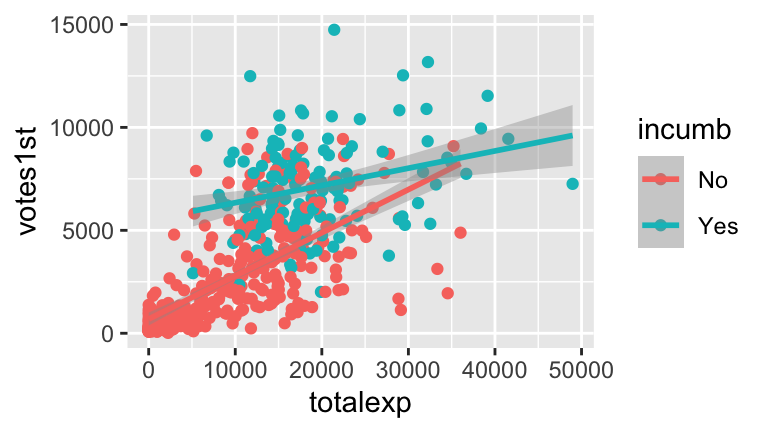


#d
#Intercept: This is the intercept for challengers.  On average, challengers that spend 0 euros receive 691 votes.    
#totalexp: This is the slope for challengers.  On average, every extra 100 euros spent corresponds to a 210 vote increase for challengers.
#incumbYes: This is the change in intercept for incumbents.  On average, incumbents that spend 0 euros will receive 4814 more votes than a challenger that spends 0 euros.
#interaction: This is the change in slope for incumbents.  On average, the increase in votes corresponding to a 100 euros increase in spending is 126 votes less for incumbents than for challengers.

age, education, industry,…

#a
cps_mod2 <- lm(wage ~ marital + age, data = cps)
summary(cps_mod2)
## 
## Call:
## lm(formula = wage ~ marital + age, data = cps)
## 
## Residuals:
##    Min     1Q Median     3Q    Max 
## -55676 -15892  -5181   9960 192894 
## 
## Coefficients:
##               Estimate Std. Error t value Pr(>|t|)    
## (Intercept)   -19595.9     3691.7  -5.308 1.18e-07 ***
## maritalsingle  -7500.1     1191.9  -6.293 3.55e-10 ***
## age             2213.9      120.8  18.331  < 2e-16 ***
## ---
## Signif. codes:  0 '***' 0.001 '**' 0.01 '*' 0.05 '.' 0.1 ' ' 1
## 
## Residual standard error: 28420 on 3166 degrees of freedom
## Multiple R-squared:  0.1569,	Adjusted R-squared:  0.1564 
## F-statistic: 294.6 on 2 and 3166 DF,  p-value: < 2.2e-16

#b
#The increase in wage with age is similar for single and married workers. So no interaction
ggplot(cps, aes(y = wage, x = age, color = marital)) + 
  geom_smooth(method="lm")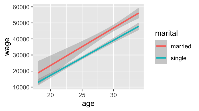


#c
#married
-19595.9 - 7500.1*0 + 2213.9*20
## [1] 24682.1
#single
-19595.9 - 7500.1*1 + 2213.9*20
## [1] 17182
#difference
24682.1 - 17182 
## [1] 7500.1

#d
#still 7500.1

cps_mod3 <- lm(wage ~ age + education + industry + marital, data = cps)
summary(cps_mod3)
## 
## Call:
## lm(formula = wage ~ age + education + industry + marital, data = cps)
## 
## Residuals:
##    Min     1Q Median     3Q    Max 
## -67652 -15101  -3072   9522 192763 
## 
## Coefficients:
##                                 Estimate Std. Error t value Pr(>|t|)    
## (Intercept)                     -52498.9     7143.8  -7.349 2.53e-13 ***
## age                               1493.4      116.2  12.855  < 2e-16 ***
## education                         3911.1      243.0  16.094  < 2e-16 ***
## industryconstruction              5659.1     6218.6   0.910    0.363    
## industryinstallation_production   1865.6     6109.3   0.305    0.760    
## industrymanagement                1476.9     6031.3   0.245    0.807    
## industryservice                  -7930.4     5945.7  -1.334    0.182    
## industrytransportation           -1084.2     6197.2  -0.175    0.861    
## maritalsingle                    -5892.8     1105.7  -5.330 1.05e-07 ***
## ---
## Signif. codes:  0 '***' 0.001 '**' 0.01 '*' 0.05 '.' 0.1 ' ' 1
## 
## Residual standard error: 26290 on 3160 degrees of freedom
## Multiple R-squared:  0.2801,	Adjusted R-squared:  0.2783 
## F-statistic: 153.7 on 8 and 3160 DF,  p-value: < 2.2e-16

#a
#12 parallel planes

#b
#married
-52498.9 + 1493.4*20 + 3911.1*16 - 7930.4*1 - 5892.8*0
## [1] 32016.3
#single
-52498.9 + 1493.4*20 + 3911.1*16 - 7930.4*1 - 5892.8*1
## [1] 26123.5
#difference
32016.3 - 26123.5
## [1] 5892.8

#c 
#married
-52498.9 + 1493.4*30 + 3911.1*12 + 5659.1*1 - 5892.8*0
## [1] 44895.4
#single
-52498.9 + 1493.4*30 + 3911.1*12 + 5659.1*1 - 5892.8*1
## [1] 39002.6
#difference
44895.4 - 39002.6
## [1] 5892.8

#d
#When controlling / holding constant age, education, and job industry, single people make $5892.8 less per year than married people (on average).

#e
#The diff in single vs married wages decrease when we control for other labor covariates.

#a
#ag = reference
table(cps$industry)
## 
##                      ag            construction installation_production 
##                      20                     170                     262 
##              management                 service          transportation 
##                    1085                    1446                     186

#b
#most = construction
#least = service

#c
#For fixed age, education, and marital status, the average yearly wage in the management industry tends to be $1476.9 higher than in the ag industry.

#subject 1 prediction
pred1 <- 136.73 + 0.015*3750
#subject 1 residual
181 - pred1
## [1] -11.98

#subject 2 prediction
pred2 <- 136.73 + 0.015*4200
#subject 2 residual
210 - pred2
## [1] 10.27

#a 
# given

#b
#residual = observed - predicted

#c
mean(penguin_mod$residual)
## [1] -4.416659e-16

#d
#this appears at the top of the model summary
summary(penguin_mod$residual)
##     Min.  1st Qu.   Median     Mean  3rd Qu.     Max. 
## -23.7626  -4.9138   0.9891   0.0000   5.1166  16.6392

#e
#This appears (approximately) as "Residual standard error" in the model summary
sd(penguin_mod$residual)
## [1] 6.903249
#a more exact calculation
dim(penguins)
## [1] 342   2
sqrt(sum(penguin_mod$residual^2)/(342 - 2))
## [1] 6.913393