13 Homework 3: Confidence intervals & bootstrapping

Directions:

• Start a new RMarkdown document.

• Load the following packages at the top of your Rmd: dplyr, ggplot2, fivethirtyeight, infer, broom.

• When interpreting visualizations, models, etc, be sure to do so in a contextually meaningful way.

• This homework is a resource for you. Record all work that is useful for your current learning & future reference. Further, try your best, but don’t stay up all night trying to finish all of the exercises! We’ll discuss any questions / material you didn’t get to tomorrow.

Goals:

In this homework you will:

• apply the concepts of confidence intervals; and

• explore new concepts in statistical inference:

  • bootstrapping;
    
  • confidence bands;
    
  • prediction bands; and
    
  • “significance”.

13.1 Warm-up

You’ve likely heard about the controversy surrounding NFL players kneeling during the national anthem. Donald Trump has publicly disagreed with the protests. This begs the question - how might fans react? To this end, fivethirtyeight article explored the association between Trump support and interest in various sports in different designated market areas. Load these data and explore the codebook.

# Load the data
data("nfl_fandom_google")

# Check out the first 6 rows
head(nfl_fandom_google)

# Examine the codebook
?nfl_fandom_google

1. Check out the data
   1. Each row represents a “designated market area” (dma). Do a little Google search and write a 1 sentence description of what this is.
      
   2. Examine and summarize the first visualization in the original fivethirtyeight article. (You’ll recreate this for “extra credit” at the end of the homework.)

2. NBA
   For now, we’ll focus on the relationship between nba interest (our response) and the trump_2016_vote (our predictor). Consider the population model represented by

   nba = \(\beta_0\) + \(\beta_1\) trump_2016_vote + \(\varepsilon\)

   where we’ll assume that \(\varepsilon \stackrel{ind}{\sim} N(0,\sigma^2)\).

   1. Construct a visualization of the relationship between nba and trump_2016_vote. Include a representation of the least squares model of this relationship.

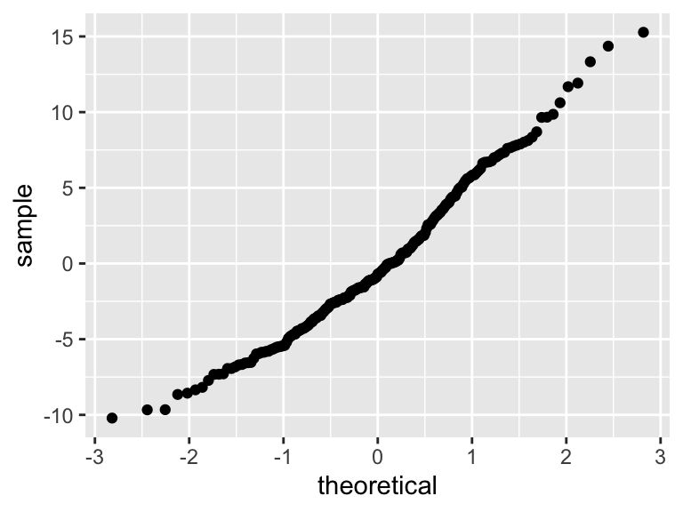
   2. Fit the least squares model, nba_mod, of nba by trump_2016_vote. (Take a second to interpret the coefficients.)

   3. Assess & comment on whether our model assumptions appear to hold.

3. Confidence intervals
   As long as the model assumptions hold (which they seem to) and our sample size of \(n=207\) is large enough (it probably is), the CLT guarantees that the sampling distribution of the estimate \(\hat{\beta}_1\) of \(\beta_1\) is \[\hat{\beta}_1 \sim N\left(\beta_1, \left(\text{s.e.}(\hat{\beta}_1)\right)^2 \right)\]
   1. Revisit the model summary table. Report the least squares estimate \(\hat{\beta}_1\) and its standard error \(\text{s.e.}(\hat{\beta}_1)\).
      
   2. Use the CLT in conjunction with the 68-95-99.7 Rule to approximate (and interpret) a 95% CI for \(\beta_1\).
      
   3. Obtain a more accurate CI using the confint() function.
      
   4. Is there enough evidence to conclude that there’s a negative association between a DMA’s NBA interest and Trump election support?

13.2 Bootstrapping

The quality of our above inference for \(\beta_1\) hinges on the CLT for the sampling distribution of \(\hat{\beta}_1\) which, in turn, hinges on satisfying the model assumptions. Thus there’s a lot of room for error - we can’t know how well the real sampling distribution of \(\hat{\beta}_1\) follows the CLT. In turn, we might be wary of the quality of the CI calculated above.

Nonparametric inferential techniques offer an alternative - they’re engineered without making any assumptions about the sampling distribution of \(\hat{\beta}_i\) (ie. no CLT!). We’ll consider one such technique: the bootstrap. The saying “to pull oneself up by the bootstraps” is often attributed to Rudolf Erich Raspe’s 1781 The Surprising Adventures of Baron Munchausen in which the character pulls himself out of a swamp by his hair (not bootstraps). Image source. In short, it means to get something from nothing, through your own effort.

We can extend the bootstrap idea to estimate the sampling distribution of \(\hat{\beta}\) using only our sample data and without making any distributional assumptions (eg: no Normal CLT). To this end, recall that the sampling distribution of \(\hat{\beta}_1\) is a collection of all possible estimates \(\hat{\beta}_1\) that we could get from all possible samples of the same size:

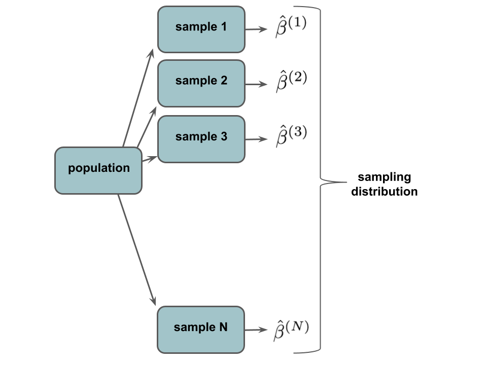
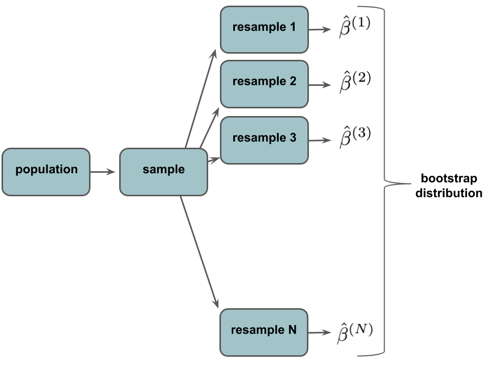
Of course, we can’t observe this in practice. We only have ONE sample from the population, thus cannot approximate the sampling distribution by taking, say, 1000 different samples from the population and calculating \(\hat{\beta}\) from each. What we can do is re-sample our sample and calculate an estimate \(\hat{\beta}_1\) from each re-sample. This produces a bootstrap distribution:

The specific bootstrapping algorithm is described below.

Bootstrapping

Suppose we’re interested in estimating some parameter \(\beta\). Then starting with our sample of size \(n\):

1. Take 1000 (many) REsamples of size \(n\) WITH REPLACEMENT from the sample. Some cases might appear multiple times, some not at all. This is analogous to seeing several similar cases in a sample from the population.

2. Calculate \(\hat{\beta}\) using each sample. This gives 1000 estimates: \[\hat{\beta}^{(1)}, ..., \hat{\beta}^{(1000)}\] The distribution of these is our bootstrap distribution. The shape and spread of this distribution (though not the location) will mimic that of the sampling distribution.

3. Use the bootstrap distribution to construct confidence intervals (and, later, hypothesis tests) for \(\beta\) WITHOUT assuming any theory about the distribution, shape, spread of the sampling distribution.

Properties:
The shape and standard deviation of the \(\hat{\beta}^{(i)}\) bootstrap distribution will provide a good approximation of the shape and standard error of the \(\hat{\beta}\) sampling distribution so long as \(n\) is “large enough” and the sample is representative of the population. However, the bootstrap distribution will be centered at our sample \(\hat{\beta}\) whereas the sampling distribution is centered at \(\beta\).

4. bootstrap simulation
   Conduct a bootstrap simulation with the following steps. (The required syntax is similar to that we used earlier!)

   • Set the random number seed to 2000.

   • Use rep_sample_n() to take 1000 resamples of \(n\) rows (market areas) from nfl_fandom_google. Be careful: don’t forget to sample with replacement.

   • For each of the 1000 samples, fit a model of nba by trump_2016_vote.

   • Output the intercept and slope coefficients for each of the 1000 models. Store these in a data frame named boot_data.

   The output might look something like this (with possibly different numbers):

   head(boot_data, 3)
   ## # A tibble: 3 x 6
   ## # Groups:   replicate [2]
   ##   replicate term            estimate std.error statistic  p.value
   ##       <int> <chr>              <dbl>     <dbl>     <dbl>    <dbl>
   ## 1         1 (Intercept)       32.6      1.79       18.2  8.12e-45
   ## 2         1 trump_2016_vote   -0.181    0.0321     -5.62 6.07e- 8
   ## 3         2 (Intercept)       34.4      1.47       23.4  9.90e-60

5. bootstrap inference: confidence intervals

   1. Create a data set, boot_slopes, that only includes the bootstrapped slopes \(\hat{\beta}_1\) (coefficient of the trump_2016_vote term).

   2. Construct and describe a histogram of the 1000 bootstrap slopes.

   3. Calculate the mean of the 1000 bootstrap slopes. (This should be close to the original least squares estimate, -0.1785322!)

   4. Calculate the standard deviation of the 1000 bootstrap slopes. Notice that this is very similar to the standard error \(\text{s.e.}(\hat{\beta}_1)\) calculated via complicated formula, 0.02891!

   5. Using only the 1000 bootstrap slopes, calculate a 95% CI for \(\beta_1\). (This should be close to what you observed for the classical approach.)
      NOTE: You weren’t given a formula to do this. Use your intuition and, subsequently, identify the appropriate function! No matter what you do, do NOT make any assumptions about normality, the CLT, etc. This means no intervals of the form ‘estimate \(\pm\) 2 (standard error)’, no use of ‘dnorm / qnorm / pnorm’, etc

6. Extending the Bootstrap
   Bootstrapping! It’s quite wonderful:

   • When the CLT is a valid assumption, bootstrap and classical results are comparable (as we saw). In cases where the CLT is suspect, a bootstrap analysis can be more reliable (at minimum, it’s a good sanity check).

   • With NO CLT assumptions, we were able to construct CIs. Thus bootstrapping is generalizable & useful in contexts for which we have limited supporting theory.

   As to the final point, consider the following. Above you bootstrapped inference for the trump_2016_vote model coefficient. Suppose instead we want to construct a bootstrap CI for the \(R^2\) of the model for nba interest vs trump_2016_vote. A complicated formula does exist for this CI. However, the quality of the CIs is sensitive to meeting the underlying theoretical assumptions about the sampling distribution for correlations. Luckily, we know how to bootstrap!

   1. Do a bootstrap simulation: for each of the 1000 resamples you constructed above, calculate the \(R^2\) between nba and trump_2016_vote. The output should look something like this (with possibly different numbers):

      head(boot_cor, 3)
      ## # A tibble: 3 x 2
      ## # Groups:   replicate [3]
      ##   replicate     x
      ##       <int> <dbl>
      ## 1         1 0.134
      ## 2         2 0.255
      ## 3         3 0.153

      HINT: From a generic lm() model, you can get the \(R^2\) by summary(my_model)$r.squared.

   2. Construct and interpret a 95% bootstrap confidence interval for the \(R^2\).

13.3 Confidence & prediction bands

Recall our original sample model of nba interest vs trump_2016_vote:

nba_mod <- lm(nba ~ trump_2016_vote, nfl_fandom_google)
summary(nba_mod)
## 
## Call:
## lm(formula = nba ~ trump_2016_vote, data = nfl_fandom_google)
## 
## Residuals:
##      Min       1Q   Median       3Q      Max 
## -10.2106  -3.6471  -0.6985   3.4572  15.2752 
## 
## Coefficients:
##                 Estimate Std. Error t value Pr(>|t|)    
## (Intercept)     32.53716    1.61583  20.136  < 2e-16 ***
## trump_2016_vote -0.17853    0.02891  -6.175 3.49e-09 ***
## ---
## Signif. codes:  0 '***' 0.001 '**' 0.01 '*' 0.05 '.' 0.1 ' ' 1
## 
## Residual standard error: 5.103 on 205 degrees of freedom
## Multiple R-squared:  0.1569,	Adjusted R-squared:  0.1527 
## F-statistic: 38.14 on 1 and 205 DF,  p-value: 3.485e-09

Consider using our original sample model to predict nba interest (\(y\)) by trump_2016_vote (\(x\)):

\[y = 32.537 - 0.179 x + \varepsilon\]

where, by the reported Residual standard error, \(\varepsilon \sim N(0, 5.103^2)\). There are 2 types of predictions we can make for, say, a Trump support of 50%:

• Model trend:
  Predict the average nba interest of all DMAs where Trump received 50% of the vote.

• Individual behavior:
  Predict the nba interest of a specific DMA (eg: Smalltown) where Trump received 50% of the vote.

The values of the two predictions are the same:

32.53716 - 0.17853 * 50
## [1] 23.61066

However, the potential error in these predictions differs. Before moving on, check your intuition: do you think there’s more error in predicting trends or individual behavior? Let’s see…

7. Confidence interval for the trend

   1. Calculate and interpret the 95% confidence interval for the average nba interest of all DMAs where Trump received 50% of the vote:

      predict(nba_mod, newdata = data.frame(trump_2016_vote = 50), interval = "confidence", level = 0.95)

      NOTE: fit is the prediction (which due to rounding is slightly different than our “by hand” prediction), lwr gives the lower bound of the CI, and upr gives the upper bound of the CI.

   2. If you have time: the CI above was constructed utilizing parametric model assumptions. Construct an alternative nonparametric bootstrap CI. (You might find some helpful syntax in HW 2.)

8. Prediction interval for an individual case

   1. Calculate and interpret the 95% prediction interval for the the nba interest of a specific DMA (eg: Smalltown) where Trump received 50% of the vote:

      predict(nba_mod, newdata = data.frame(trump_2016_vote = 50), interval = "prediction", level = 0.95)

   2. If you have time: Construct an alternative nonparametric bootstrap prediction interval. HINT: You can use rnorm(1, mean = 0, sd = 5.103) to simulate a Normal residual / individual variability from the trend.

9. Visualizing confidence & prediction bands
   We can visualize these concepts by placing prediction and confidence bands around the entire model. These represent the intervals calculated at each value of the trump_2016_vote variable. To begin, construct confidence bands by omitting se = FALSE in the geom_smooth():

   # Confidence bands
   ggplot(nfl_fandom_google, aes(y = nba, x = trump_2016_vote)) + 
       geom_point() + 
       geom_smooth(method = "lm")

   Next, include prediction bands using this more complicated syntax:

   # Calculate prediction intervals for every trump_2016_vote value
   pred_int_1 <- data.frame(nfl_fandom_google, predict(nba_mod, 
       newdata = data.frame(trump_2016_vote = nfl_fandom_google$trump_2016_vote), interval = 'prediction'))
   head(pred_int_1)    
   
   # Prediction bands
   ggplot(pred_int_1, aes(y = nba, x = trump_2016_vote)) + 
       geom_point() + 
       geom_smooth(method='lm', color="black") + 
       geom_ribbon(aes(y=fit, ymin=lwr, ymax=upr, fill='prediction'), 
   alpha=0.2)

   Explain:

   1. Why is it intuitive that the prediction bands are wider than the confidence bands?
      
   2. Though it’s not as noticeable with the prediction bands, these and the confidence bands are always the most narrow at the same point – in this case the coordinates are (22.8, 54.5). What other meaning do these values have? Provide some proof and explain why it makes intuitive sense that the bands are narrowest at this point.

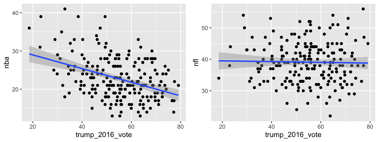
10. Toward hypothesis testing
    Tomorrow we’ll start talking about hypothesis testing. We already have the tools and ideas to do some simple tests. Consider the below plots of nba and nfl interest vs trump_2016_vote. Do we have enough evidence to conclude there’s a relationship between a market’s NBA interest & their Trump support? What about the relationship between a market’s NFL interest & their Trump support? Explain.
    

13.4 Extra

Recreate the visualization at the top of the fivethirtyeight article. To get started, you’ll first need to reshape the data so that instead of each row representing a DMA, each row represents a DMA & sport combination:

nfl_fandom_google %>% 
    gather(activity, market_share, -c(dma, trump_2016_vote))

13.5 HW3 solutions

Don’t peak until and unless you really, really need to!

1. Check out the data
   

1. A “region where the population can receive the same (or similar) television and radio station offerings, and may also include other types of media including newspapers and Internet content.”

2. In terms of politics, NBA interest is most associated with “blue” market areas, college football is most associated with “red” market areas, and the NFL is pretty neutral.

2. NBA

#a
ggplot(nfl_fandom_google, aes(x=trump_2016_vote, y=nba)) + 
    geom_point() + 
    geom_smooth(method="lm")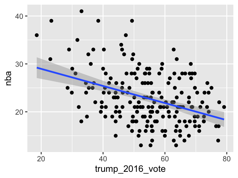

#b
nba_mod <- lm(nba ~ trump_2016_vote, nfl_fandom_google)
summary(nba_mod)
## 
## Call:
## lm(formula = nba ~ trump_2016_vote, data = nfl_fandom_google)
## 
## Residuals:
##      Min       1Q   Median       3Q      Max 
## -10.2106  -3.6471  -0.6985   3.4572  15.2752 
## 
## Coefficients:
##                 Estimate Std. Error t value Pr(>|t|)    
## (Intercept)     32.53716    1.61583  20.136  < 2e-16 ***
## trump_2016_vote -0.17853    0.02891  -6.175 3.49e-09 ***
## ---
## Signif. codes:  0 '***' 0.001 '**' 0.01 '*' 0.05 '.' 0.1 ' ' 1
## 
## Residual standard error: 5.103 on 205 degrees of freedom
## Multiple R-squared:  0.1569,	Adjusted R-squared:  0.1527 
## F-statistic: 38.14 on 1 and 205 DF,  p-value: 3.485e-09

#c 
# The assumptions appear to hold

ModResults <- data.frame(predicted=nba_mod$fitted.values, residual=nba_mod$residuals)

# A plot of residuals versus the predictions    
ggplot(ModResults, aes(y=residual, x=predicted)) + 
    geom_point() + 
    geom_hline(yintercept=0)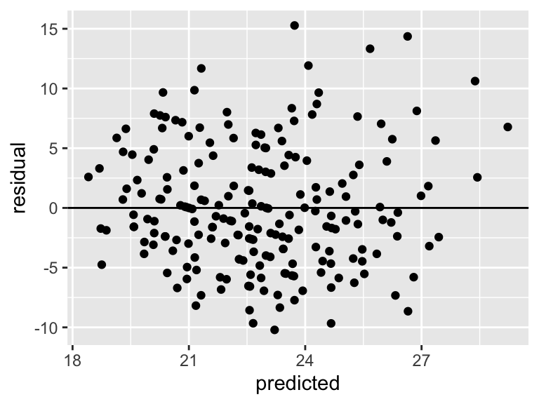

    
# A Q-Q plot of the residuals
ggplot(ModResults, aes(sample=residual)) + 
    geom_qq()

3. Confidence intervals

sqrt((1/207 * sum(ModResults$residual^2)) / sum((nfl_fandom_google$trump_2016_vote - mean(nfl_fandom_google$trump_2016_vote))^2))
## [1] 0.02876981

1. \(\hat{\beta}_1\) = -0.17853, \(\text{s.e.}(\hat{\beta}_1)\) = 0.02891

2. \(\hat{\beta}_1 \pm 2\text{s.e.}(\hat{\beta}_1) = -0.17853 \pm 2*0.02891 = (-0.23635, -0.12071)\)

3. .

confint(nba_mod)
##                      2.5 %     97.5 %
## (Intercept)     29.3513722 35.7229399
## trump_2016_vote -0.2355309 -0.1215335

4. Yes. We’re 95% confident that, for every extra percentage point increase in Trump’s vote, the average decrease in NBA interest is between 0.12 and 0.24 percentage points.

4. bootstrap simulation

set.seed(2000)

resamples <- rep_sample_n(nfl_fandom_google, size = 207, reps = 1000, replace = TRUE)

boot_data <- resamples %>% 
    group_by(replicate) %>% 
    do(lm(nba ~ trump_2016_vote, data=.) %>% tidy())    

head(boot_data, 3)
## # A tibble: 3 x 6
## # Groups:   replicate [2]
##   replicate term            estimate std.error statistic  p.value
##       <int> <chr>              <dbl>     <dbl>     <dbl>    <dbl>
## 1         1 (Intercept)       32.6      1.79       18.2  8.12e-45
## 2         1 trump_2016_vote   -0.181    0.0321     -5.62 6.07e- 8
## 3         2 (Intercept)       34.4      1.47       23.4  9.90e-60

5. bootstrap inference: confidence intervals

#a 
boot_slopes <- boot_data %>% 
    filter(term == "trump_2016_vote")
    
#b
ggplot(boot_slopes, aes(x = estimate)) +
    geom_histogram()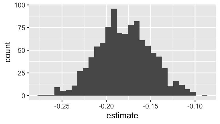    

#c
mean(boot_slopes$estimate)
## [1] -0.1800603

#d
sd(boot_slopes$estimate)
## [1] 0.03052984

#e 
# Just take the 2.5th & 97.5th quantiles
quantile(boot_slopes$estimate, c(0.025,0.975))
##       2.5%      97.5% 
## -0.2376915 -0.1191649

6. Extending the Bootstrap

#a
boot_cor <- resamples %>% 
    group_by(replicate) %>% 
    do(summary(lm(nba ~ trump_2016_vote, data = .))$r.squared %>% tidy()) 

head(boot_cor, 3)
## # A tibble: 3 x 2
## # Groups:   replicate [3]
##   replicate     x
##       <int> <dbl>
## 1         1 0.134
## 2         2 0.255
## 3         3 0.153


#b
#We're 95% confident that the R^2 is between 7.7 and 24.8%
quantile(boot_cor$x, c(0.025,0.975))
##       2.5%      97.5% 
## 0.07471559 0.25973730

7. Confidence interval for the trend

#a 
predict(nba_mod, newdata = data.frame(trump_2016_vote = 50), interval = "confidence", level = 0.95)
##        fit      lwr      upr
## 1 23.61055 22.86515 24.35594

#b
boot_CI <- resamples %>% 
    group_by(replicate) %>% 
    do(lm(nba ~ trump_2016_vote, data = .) %>% 
        predict(., newdata = data.frame(trump_2016_vote = 50)) %>% tidy())
quantile(boot_CI$x, c(0.025,0.975))
##     2.5%    97.5% 
## 22.79113 24.42996

8. Prediction interval for an individual case

#a
predict(nba_mod, newdata = data.frame(trump_2016_vote = 50), interval = "prediction", level = 0.95)
##        fit      lwr      upr
## 1 23.61055 13.52231 33.69878

#b
boot_CI <- boot_CI %>% 
    mutate(pred = x + rnorm(1, 0, 5.103))
quantile(boot_CI$pred, c(0.025,0.975))
##     2.5%    97.5% 
## 14.06698 33.18374

9. Visualizing confidence & prediction bands

# Confidence bands
ggplot(nfl_fandom_google, aes(y = nba, x = trump_2016_vote)) + 
    geom_point() + 
    geom_smooth(method = "lm")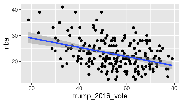

# Calculate prediction intervals for every trump_2016_vote value
pred_int_1 <- data.frame(nfl_fandom_google, predict(nba_mod, 
    newdata = data.frame(trump_2016_vote = nfl_fandom_google$trump_2016_vote), interval = 'prediction'))
head(pred_int_1)    
##                          dma nfl nba mlb nhl nascar cbb cfb trump_2016_vote
## 1      Abilene-Sweetwater TX  45  21  14   2      4   3  11           79.13
## 2                  Albany GA  32  30   9   1      8   3  17           59.12
## 3 Albany-Schenectady-Troy NY  40  20  20   8      6   3   4           44.11
## 4    Albuquerque-Santa Fe NM  53  21  11   3      3   4   6           39.58
## 5              Alexandria LA  42  28   9   1      5   3  12           69.64
## 6                  Alpena MI  28  13  21  12     10   7   9           63.61
##        fit       lwr      upr
## 1 18.40990  8.227957 28.59185
## 2 21.98233 11.894008 32.07065
## 3 24.66210 14.559700 34.76450
## 4 25.47085 15.349989 35.59171
## 5 20.10417  9.982531 30.22581
## 6 21.18072 11.082519 31.27892

# Prediction bands
ggplot(pred_int_1, aes(y = nba, x = trump_2016_vote)) + 
    geom_point() + 
    geom_smooth(method='lm', color="black") + 
    geom_ribbon(aes(y=fit, ymin=lwr, ymax=upr, fill='prediction'), 
alpha=0.2)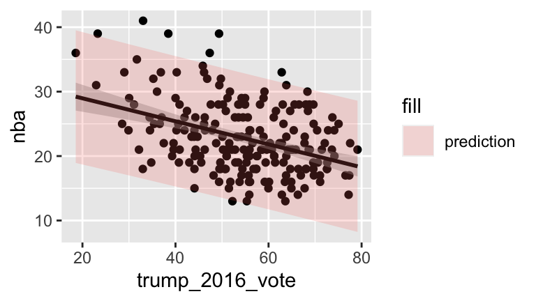

1. Intuitively, it’s harder to predict individual behavior than average behavior / trend. Mathematically, when predicting trend, we don’t have to incorporate variability in residuals \(\varepsilon\) - we do need to when predicting individual behavior.
   
2. These are the means of the response & predictor.

nfl_fandom_google %>% 
summarize(mean(trump_2016_vote), mean(nba))
## # A tibble: 1 x 2
##   `mean(trump_2016_vote)` `mean(nba)`
##                     <dbl>       <dbl>
## 1                    54.5        22.8