6 Evaluating models
One of the most famous quotes in statistics is the following from George Box (1919–2013):
“All models are wrong, but some are useful.”
Thus far, we’ve constructed models from sample data & used these to tell stories about the relationships among variables of interest. We haven’t yet discussed the quality of these models. To this end, it’s important to ask the following.
Model evaluation questions
- How fair is our model?
- How wrong is our model?
- How strong is our model? How well does it explain the variability in the response?
- How accurate are our model’s predictions?
Though these questions are broadly applicable across all machine learning techniques, we’ll examine these questions in the linear regression context
\[Y = \beta_0 + \beta_1 X_{1} + \beta_2 X_{2} + \cdots + \beta_k X_{k} + \varepsilon \; .\]
applied to a specific example. The body_data includes measurements on 40 adults:
body_data <- read.csv("https://www.macalester.edu/~ajohns24/data/bodyfat50.csv")
body_data <- body_data %>%
  select(-fatBrozek, -density, -fatFreeWeight, -hipin, -forearm, -neck, -adiposity) %>%
  filter(ankle < 30)
Our overall goal will be to model \(Y\), body fat percentage (fatSiri). To begin, we’ll model \(Y\) by \(X_1\), a person’s chest circumference (chest):
model_1 <- lm(fatSiri ~ chest, body_data)
ggplot(body_data, aes(x = chest, y = fatSiri)) +
  geom_point() +
  geom_smooth(method = "lm", se = FALSE)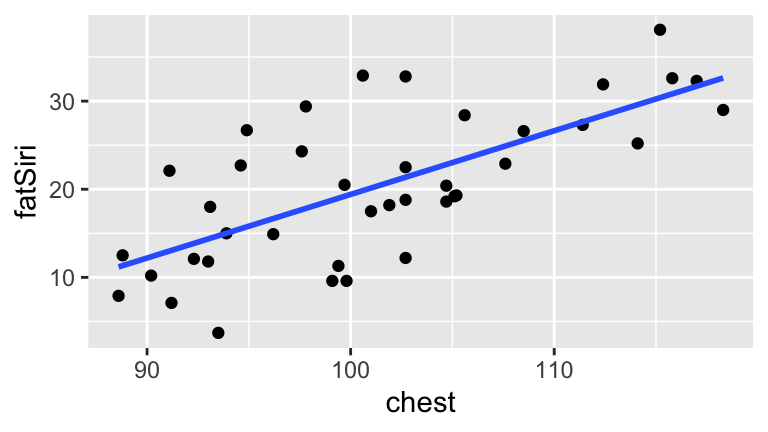
6.1 How FAIR is our model?
It’s critical to ask whether our model is fair:
- Who collected the data / who funded the data collection?
- How did they collect the data?
- Why did they collect the data?
- What are the implications of the analysis on individuals and society?
Examples of unfair models (or “algorithms”) unfortunately abound:
- Amazon’s resume filter discriminated against women applicants
- Facial recognition models, increasingly being used in police surveillance, are more likely to misidentify non-white subjects
- ICEs algorithm disproportionately recommended detention
- Is our model fair?
6.2 How WRONG is our model?
In asking whether our model is wrong, we’re specifically asking: what assumptions does our model make and are these reasonable? There are 2 key assumptions behind our normal linear regression models:
- Assumption 1:
The observations of (\(Y,X_1,X_2,...,X_k\)) for any case are independent of the observations for any other case. (This would be violated if we had multiple observations or rows of data for each subject or if the data were a time series or…) - Assumption 2:
At any set of predictor values \((X_{1}^*, X_{2}^*, \ldots, X_{k}^*)\),
\[\varepsilon \sim N(0,\sigma^2)\]
More details are provided in the “Wrapping Up” section below. For now, we’ll focus on some intuition.
To determine how wrong our model might be, we can perform a residual analysis. Specifically, we can plot the residuals vs the predicted / fitted values. What we want to see is a random distribution of the residuals around 0 with no apparent patterns. Why are patterns bad? They would indicate that our model is systematically missing the trend in the relationship between \(Y\) and the \(X_i\).
- Intuition
For the plots below, use the raw data (top row) and corresponding residual plots (bottom row) to determine whether the following models are wrong.

Is our model wrong?
# Residual plot
ggplot(model_1, aes(x = .fitted, y = .resid)) +
  geom_point() +
  geom_hline(yintercept = 0)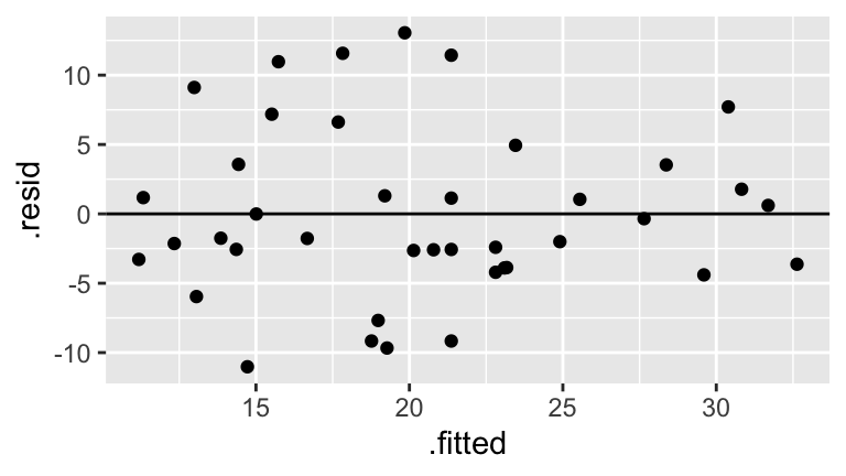
6.3 How STRONG is our model?
Meeting the model assumptions isn’t the only important piece of the model evaluation process. We also need a sense of the model’s strength in explaining \(Y\):
Three models
Consider three possible models offatSiri. Which of these do you anticipate will be the strongest?model_1 <- lm(fatSiri ~ chest, body_data) model_2 <- lm(fatSiri ~ age, body_data) model_3 <- lm(fatSiri ~ age + chest, body_data)ggplot(body_data, aes(x = chest, y = fatSiri)) + geom_point() ggplot(body_data, aes(x = age, y = fatSiri)) + geom_point() ggplot(body_data, aes(x = age, y = fatSiri, size = chest)) + geom_point()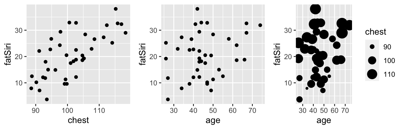
Measuring strength with R2
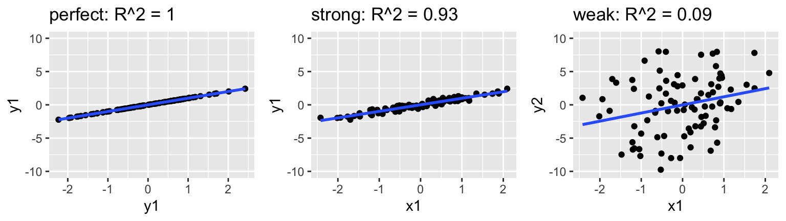
\(R^2 \in [0,1]\) measures the proportion of the variability in \(Y\) that’s explained by the model. Thus an \(R^2\) of 0 indicates that the model doesn’t explain any of the variability in \(Y\); an \(R^2\) of 1 indicates that the model perfectly explains the variability in \(Y\). See the plots at the top of this section for reference. Mathematically, let \(\overline{y} = \frac{1}{n} \sum_{i=1}^n y_i\) denote the sample mean of the observed \(Y\) values and \(\hat{y}_i\) denote the model prediction of \(y_i\). Then\[R^2 = \frac{\text{Var}(\text{predictions})}{\text{Var}(y)} = \frac{\sum_{i=1}^n(\hat{y}_i - \overline{y}_i)^2}{\sum_{i=1}^n(y_i - \overline{y})^2}\]
Equivalently,
\[R^2 = 1 - \frac{\text{Var}(\text{residuals})}{\text{Var}(y)} = 1 - \frac{\sum_{i=1}^n(y_i - \hat{y}_i)^2}{\sum_{i=1}^n(y_i - \overline{y})^2}\]
We could calculate \(R^2\) by hand, but won’t. It’s reported in the model
summary()table underMultiple R-squared:Which of the three models is strongest?
In general, what do you think happens to \(R^2\) as we add more predictors to the model?
6.4 How ACCURATE are our predictions?
Like the question of overall model strength, the question of a model’s accuracy is directly linked to the size of its residuals:
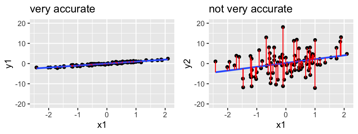
To this end we can summarize the combined size of the residuals, \(y_1 - \hat{y}_1\), \(y_2 - \hat{y}_2\), …, \(y_n - \hat{y}_n\) where \(n\) is sample size. There are multiple metrics, but we’ll focus on MAE:
\[\begin{split} \text{MAE} & = \text{ mean absolute error } = \frac{1}{n}\sum_{i=1}^n |y_i - \hat{y}_i| \\ \text{MSE} & = \text{ mean squared error } = \frac{1}{n}\sum_{i=1}^n (y_i - \hat{y}_i)^2 \\ \text{RMSE} & = \text{ root mean squared error } = \sqrt{MSE} \\ \end{split}\]
- Measuring predictive accuracy
Calculate and interpret the MAE for our three models.
Which model produces the most accurate predictions?
In general, what do you think happens to MAE (and RMSE and MSE) as we add more predictors to the model?
Though it might be tempting to evaluate predictive accuracy by calculating the mean residual, explain why this wouldn’t work. Provide some numerical evidence.
6.5 Pause for an experiment
Each breakout room will be given their own set of body fat data that includes measurements on 40 adults:
As a group, use your data to choose which of the following you believe to be the best predictive model of
fatSiri:- Model 1:
fatSiri ~ chest
- Model 2:
fatSiri ~ chest + age
- Model 3:
fatSiri ~ chest * age * weight * height * abdomen
- Model 1:
Only when you’re done:
- Open this Top Model Competition Google Doc.
- Record your team name & the number of the data you were given.
- Record which model you chose (1, 2, or 3).
- Record the MAE for your model.
- Open this Top Model Competition Google Doc.
Don’t peak until the instructor gives all students the go ahead
What do you know?! 40 new people just walked into the doctor’s office and the doctor wants to predict their fatSiri.
How well does your model do in the real world? Use your model to predict() fatSiri for these 40 new subjects and, subsequently, calculate the MAE for the new patients. (Take note of how the code changes here!)
# Import the new data
new_patients <- read.csv("https://www.macalester.edu/~ajohns24/data/bodyfat182.csv")

# Predict fatSiri & compute MAE
new_patients %>%
  mutate(prediction = predict(your_model, newdata = new_patients)) %>%
  summarize(mean(abs(fatSiri - prediction)))
Record your MAE in the Google sheet. Relative to its predictive accuracy on the new subjects, which group had the best model? What’s the central theme here?
6.6 Cross validation
Our post-experiment discussions highlight a couple of important themes:
Training and testing our model using the same data can result in overly optimistic assessments of model quality. For example, in-sample or training errors (ie. MAE calculated using the same data that we used to train the model) are often smaller than testing errors (ie. MAE calculated using data not used to train the model).
Adding more and more predictors to a model might result in overfitting the model to the noise in our sample data. In turn, the model loses the broader trend and does not generalize to new data outside our sample (ie. it results in bad predictions).
Example: the concept
Self-driving cars must build algorithms / models which can identify humans. If our data consisted of the image below3, what would be the consequences of using the following model: Identify as human if it has…- a head, a nose
- AND has arms down at the sides, doesn’t smile, is facing forward, appears in groups of 7, has an eastern shadow,…

- a head, a nose
We’ll consider a different measure of predictive accuracy that addresses some of these concerns: cross validation. Throughout this discussion, we’ll all use the same data and compare the following 2 models:
# Plot the models
ggplot(body_data, aes(y = fatSiri, x = chest)) +
    geom_point() +
    stat_smooth(method="lm", se=FALSE)

ggplot(body_data, aes(y = fatSiri, x = chest)) +
    geom_point() +
    stat_smooth(method="lm", formula=y~poly(x, 16), se=FALSE)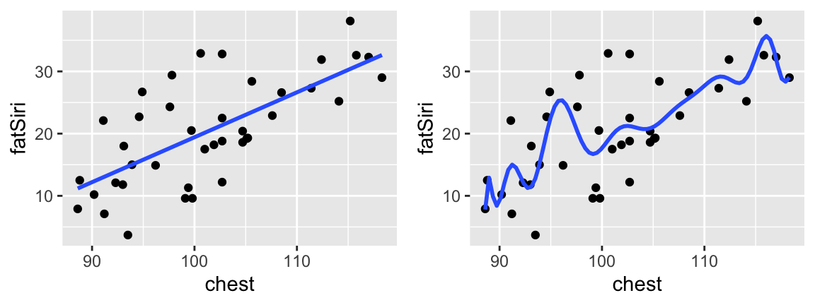
The in-sample MAE for these 2 models follows:
# MAE for model_1
mean(abs(model_1$residuals))
## [1] 4.836629

# MAE for model_2
mean(abs(model_16$residuals))
## [1] 4.070526
NOTE
Though model_16 has a better (lower) MAE than model_1, it might be overfit to our sample data. That is, it does a great job of picking up the little trends in our data but might not generalize well to new data.
Validation
In practice, we only have one sample of data. We need to use this one sample to both train (build) and test (evaluate) our model. Consider a simple strategy where we randomly select half of the sample to train the model and test the model on the other half. To ensure that we all get the same samples and can reproduce our results, we’ll set the random number generating seed to the same number (2000). We’ll discuss this in detail as a class!# Set the random number seed set.seed(2000) # Randomly sample half of these for training data_train <- body_data %>% sample_frac(0.5) # Take the the other 20 for testing data_test <- body_data %>% anti_join(., data_train) # Confirm the dimensions dim(data_train) ## [1] 20 12 dim(data_test) ## [1] 20 12Using the training data: Fit the model of
fatSiribychestand calculate the training MAE.How well does this model generalize to the test set? Use the training model to predict
fatSirifor the test cases and calculate the resulting test MAE. This should equal 4.855822. NOTE: This code is more complicated than calculating the training MAE. Since the test cases aren’t part of the training data, we can’t just grab their residuals frommodel_1_train– we have to actually calculate them.Notice that, as we might expect, the testing MAE (4.855822) is greater than the training MAE (4.698395). We could stop here use this testing MAE to communicate / measure how well
model_1generalizes to the population. But what might be the flaws in this approach? Can you think of a better idea?
Solution
# Construct the training model model_1_train <- lm(fatSiri ~ chest, data_train) # Calculate the training MAE mean(abs(model_1_train$residuals)) ## [1] 4.698395 # b data_test %>% mutate(predictions = predict(model_1_train, newdata = .)) %>% summarize(mean(abs(fatSiri - predictions))) ## mean(abs(fatSiri - predictions)) ## 1 4.855822- First, these comparisons are based on the training and test sets we happened to get. If we chose new training and test sets, we would get different answers! Second, we’re only using half of the data to train the model, thus are losing so much info and will likely overestimate error as a result.
2-fold cross validation
The validation approach we used above useddata_trainto build the model and then tested this model ondata_test. Let’s reverse the roles!# Build the model using data_test model_1_test <- lm(fatSiri ~ chest, ___) # Test the model on data_train ___ %>% mutate(predictions = predict(model_1_test, newdata = .)) %>% summarize(mean(abs(fatSiri - predictions)))We now have 2 measures of MAE after reversing the roles of training and testing: 4.855822 and 6.129452. Instead of picking either one of these measures, average them to get an estimate of the 2-fold cross validation error. The general k-fold cross validation algorithm is described below.
Solution
\(k\)-Fold Cross Validation (CV)
Divide the data into \(k\) groups / folds of equal size.
Repeat the following procedures for each fold \(j \in \{1,2,...,k\}\):
- Divide the data into a test set (fold \(j\)) & training set (the other \(k-1\) folds).
- Fit a model using the training set.
- Use this model to predict the responses for the \(n_j\) cases in fold \(j\): \(\hat{y}_1, ..., \hat{y}_{n_j}\)
- Calculate the MAE for fold \(j\): \[\text{MAE}_j = \frac{1}{n_j}\sum_{i=1}^{n_j} (y_i - \hat{y}_i)^2\]
Calculate the “cross validation error”, ie. the average MAE from the \(k\) folds: \[\text{CV}_{(k)} = \frac{1}{k} \sum_{j=1}^k \text{MAE}_j\]
In pictures: 10-fold CV

Picking \(k\)
To implement \(k\)-fold CV, we have to pick a value of \(k\) in \(\{2,3,...,n\}\) where \(n\) is the original sample size.- \(n\)-fold CV is also called “leave-one-out CV” (LOOCV). Explain why.
- In practice, \(k=10\) and \(k=7\) are common choices for cross validation. What advantages do you think 10-fold CV has over 2-fold CV? What advantages do you think 10-fold CV has over LOOCV?
Solution
- Each fold contains only 1 case / row. Thus when we leave out that fold for testing, we’re leaving 1 out!
- 2-fold only uses 50% of the data for training, thus might overestimate error. LOOCV is computationally expensive – we have to build \(n\) models (1 per training fold) vs 10 models
caret package
We could but won’t hard code our own CV metrics. Instead, we’ll use thecaretpackage. This powerful package allows us to streamline the vast world of machine learning tools into one common syntax. Though we’ll only usecaretfor linear regression models (lm), check out the different machine learningmethods that we can utilize incaret.Use the following code to re-run
model_1andmodel_16with CV. Examine the code:Check out the summaries. These are the same as when we used
lm():
Solution
library(caret) # Model 1 model_1_redo <- train( fatSiri ~ chest, data = body_data, method = "lm", trControl = trainControl(method = "cv", number = 10) ) # Model 16 (you do) model_16_redo <- train( fatSiri ~ poly(chest, 16), data = body_data, method = "lm", trControl = trainControl(method = "cv", number = 10) ) summary(model_1_redo) ## ## Call: ## lm(formula = .outcome ~ ., data = dat) ## ## Residuals: ## Min 1Q Median 3Q Max ## -11.021 -3.689 -1.763 3.540 13.052 ## ## Coefficients: ## Estimate Std. Error t value Pr(>|t|) ## (Intercept) -52.7946 12.3247 -4.284 0.000121 *** ## chest 0.7221 0.1212 5.958 6.5e-07 *** ## --- ## Signif. codes: 0 '***' 0.001 '**' 0.01 '*' 0.05 '.' 0.1 ' ' 1 ## ## Residual standard error: 6.215 on 38 degrees of freedom ## Multiple R-squared: 0.483, Adjusted R-squared: 0.4694 ## F-statistic: 35.5 on 1 and 38 DF, p-value: 6.5e-07 summary(model_16_redo) ## ## Call: ## lm(formula = .outcome ~ ., data = dat) ## ## Residuals: ## Min 1Q Median 3Q Max ## -10.3586 -2.5157 -0.0898 3.1709 13.9473 ## ## Coefficients: ## Estimate Std. Error t value Pr(>|t|) ## (Intercept) 20.4025 1.1381 17.926 5.18e-15 *** ## `poly(chest, 16)1` 37.0315 7.1982 5.145 3.26e-05 *** ## `poly(chest, 16)2` 0.8425 7.1982 0.117 0.908 ## `poly(chest, 16)3` 2.5596 7.1982 0.356 0.725 ## `poly(chest, 16)4` -6.3759 7.1982 -0.886 0.385 ## `poly(chest, 16)5` -4.7048 7.1982 -0.654 0.520 ## `poly(chest, 16)6` 1.4002 7.1982 0.195 0.847 ## `poly(chest, 16)7` -2.8931 7.1982 -0.402 0.691 ## `poly(chest, 16)8` -3.7131 7.1982 -0.516 0.611 ## `poly(chest, 16)9` 4.6820 7.1982 0.650 0.522 ## `poly(chest, 16)10` -4.6029 7.1982 -0.639 0.529 ## `poly(chest, 16)11` 1.6628 7.1982 0.231 0.819 ## `poly(chest, 16)12` 8.2036 7.1982 1.140 0.266 ## `poly(chest, 16)13` -1.0978 7.1982 -0.153 0.880 ## `poly(chest, 16)14` -3.4796 7.1982 -0.483 0.633 ## `poly(chest, 16)15` 6.4903 7.1982 0.902 0.377 ## `poly(chest, 16)16` -3.6733 7.1982 -0.510 0.615 ## --- ## Signif. codes: 0 '***' 0.001 '**' 0.01 '*' 0.05 '.' 0.1 ' ' 1 ## ## Residual standard error: 7.198 on 23 degrees of freedom ## Multiple R-squared: 0.5803, Adjusted R-squared: 0.2883 ## F-statistic: 1.987 on 16 and 23 DF, p-value: 0.0647
CV
We can also get the CV MAE from the caret package:Recall that
model_1had an in-sample MAE of 4.84 andmodel_16had an in-sample MAE of 4.07- Within both models, how do the in-sample errors compare to the CV errors?
- Which model has the best in-sample errors? The best CV error?
- Which model would you choose?
Solution
model_1_redo$results ## intercept RMSE Rsquared MAE RMSESD RsquaredSD MAESD ## 1 TRUE 5.754134 0.6119259 4.965074 2.587765 0.2845463 2.445648 model_16_redo$results ## intercept RMSE Rsquared MAE RMSESD RsquaredSD MAESD ## 1 TRUE 208.7418 0.3616469 108.8588 586.752 0.3127704 294.1558- In-sample MAE was higher
- model_16 had the best in-sample MAE. model_1 has the best CV MAE.
- model_1
Digging deeper
model_1_redo$resultsgives the final CV MAE, or the average MAE across all 10 test folds. In contrast,model_1_redo$resampleprovides the MAE from each test fold, thus more detailed info. Try to calculatemodel_1_redo$resultsfrom themodel_1_redo$resampleinformation.
Solution
Parsimonious Models
Reflecting back, these exercises illustrate the importance of parsimony in a statistical analysis. A parsimonious analysis is one that balances simplicity with the desire for the highest \(R^2\) (for example). In the case of model building, increasing the number of predictors increases \(R^2\). BUT:
The greater the number of predictors, the more complicated the model is to implement and interpret;
The greater the number of predictors, the greater the risk of overfitting the model to our particular sample of data. That is, the greater the risk of our model losing the general trend, hence, the model’s generalizability to the greater population.
6.7 Wrapping up
6.7.1 Resources
For more detail, you can watch the following videos. These were made for another course, but are still relevant to this bootcamp.
6.7.2 Details behind model assumptions
There are 2 key assumptions behind our normal linear regression models:
- Assumption 1:
The observations of (\(Y,X_1,X_2,...,X_k\)) for any case are independent of the observations for any other case. - Assumption 2:
At any set of predictor values \((X_{1}^*, X_{2}^*, \ldots, X_{k}^*)\),
\[\varepsilon \sim N(0,\sigma^2)\] That is:the expected value of the residuals is \(E(\varepsilon) =0\)
In words: Across the entire model, responses are balanced above & below the trend. Thus the model accurately describes the “shape” and “location” of the trend.homoskedasticity: the variance of the residuals \(Var(\varepsilon) = \sigma^2\)
In words: Across the entire model, variability from the trend is roughly constant.the \(\varepsilon\) are normally distributed
In words: individual responses are normally distributed around the trend (closer to the trend and then tapering off)
Residual Analysis Summary
Assumption Consequence Diagnostic Solution independence inaccurate inference common sense / context use a different modeling technique \(E(\varepsilon)=0\) lack of model fit plot of residuals vs predictions transform \(x\) and/or \(y\) \(Var(\varepsilon)=\sigma^2\) inaccurate inference plot of residuals vs predictions transform \(y\) normality of \(\varepsilon\) if extreme, inaccurate inference Q-Q plot if extreme, transform \(y\)
.png)