12 Homework 2: Data wrangling & model evaluation
Directions:
Start a new RMarkdown document.
Load the following packages at the top of your Rmd:
dplyr,ggplot2,leaps,caret,lubridate,mosaicData(you might need to install some of these first)This homework is a resource for you. Record all work that is useful for your current learning & future reference. Further, try your best, but don’t stay up all night trying to finish all of the exercises! We’ll discuss any questions / material you didn’t get to tomorrow.
Goals:
In this homework you will practice two pieces in the machine learning workflow: data cleaning & model (algorithm) building:

Specifically, you will:
practice your data wrangling & model evaluation skills; and
explore new concepts in the iterative process of model building & model evaluation:
- multicollinearity;
- model selection; and
- bias-variance trade-off.
- multicollinearity;
12.1 Data wrangling practice
The number of daily births in the US varies over the year and from day to day. What’s surprising to many people is that the variation from one day to the next can be huge: some days have only about 80% as many births as others. Why? In this section we’ll use basic data wrangling skills to understand some drivers of daily births.
The data table Birthdays in the mosaicData package gives the number of births recorded on each day of the year in each state from 1969 to 1988.4
data("Birthdays")
head(Birthdays, 3)
##   state year month day       date wday births
## 1    AK 1969     1   1 1969-01-01  Wed     14
## 2    AL 1969     1   1 1969-01-01  Wed    174
## 3    AR 1969     1   1 1969-01-01  Wed     78
- Minnesota
Create a data set with only births in Minnesota (MN) in 1980, and sort the days from those with the most births to those with the fewest. Show the first 6 rows.
- Averaging births
Usedplyrverbs to calculate the following.- The average number of daily births (across all years and states).
- The average number of daily births in each year (across all states).
- The average number of daily births in each year, by state. (You don’t have to print all rows.)
- The average number of daily births (across all years and states).
- Working with dates
For the remainder of this analysis, we’ll work with data aggregated across the states.- Create a new data set,
daily_births, that adds up the total number of births in the U.S. on each day (across all the states). Your table should have 7305 rows and 2 columns.
- The
daily_birthscolumns includedate. Thoughdateappears in a human-readable way, it’s actually in a format (calledPOSIXdate format) that automatically respects the order of time. Thelubridatepackage contains helpful functions that extract various information about dates. These include:5(http://r4ds.had.co.nz/dates-and-times.html) ]year()month()— a number 1-12 or, with the argumentlabel = TRUE, a string (Jan,Feb, …)week()— a number 1-53yday()— “Julian” day of the year, a number 1-366mday()— day of the month, a number 1-31wday()— weekday as a number 1-7 or, with the argumentlabel = TRUE, a string (Sun,Mon,…)
lubridatefunctions, add 4 new variables (columns) todaily_births: year, month (string), day of the month, and weekday (string). Here’s what the data should look like with our new columns:
Table 12.1: Aggregated births data with additional variables. date total year month mday weekday 1969-01-01 8486 1969 Jan 1 Wed 1969-01-02 9002 1969 Jan 2 Thu 1969-01-03 9542 1969 Jan 3 Fri 1969-01-04 8960 1969 Jan 4 Sat 1969-01-05 8390 1969 Jan 5 Sun 1969-01-06 9560 1969 Jan 6 Mon - Create a new data set,
- Seasonality
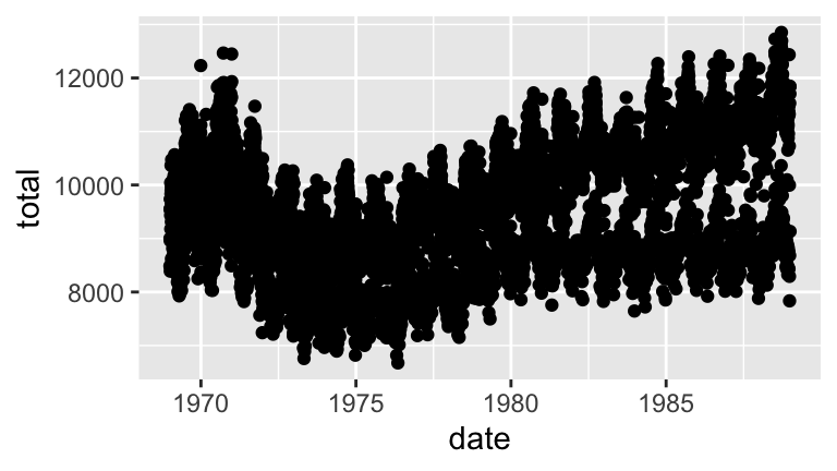
Using yourdaily_birthsdata…- Plot daily births (y axis) vs date (x axis). Comment.
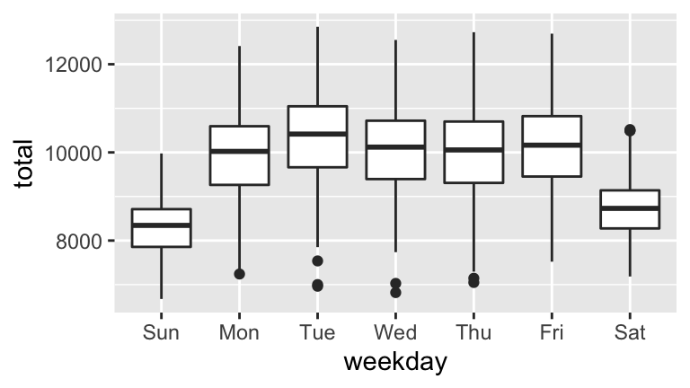
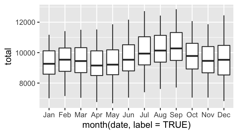
- Digging deeper into the observed seasonality, construct 2 separate visualizations of: births by day of the week and births by month.
- Summarize your observations. When are the most babies born? The fewest?
- Sleuthing
In your plot of daily births vs date in the previous exercise (part a), one goofy thing stands out: there seem to be 2-3 distinct groups of points.- To zoom in on the pattern, create a new subset of
daily_birthswhich only includes the 2 year span from 1980-81. - Using the 1980-81 data, plot daily births vs date and add a layer that explains the distinction between the distinct groups.
- There are some exceptions to the rule in part b, ie. some cases that should belong to group 1 but behave like the cases in group 2. Explain why these cases are exceptions - what explains the anomalies / why these are special cases?
- To zoom in on the pattern, create a new subset of
- Superstition
Some people are superstitious about Friday the 13th.- Create a new data set,
friday_only, that only contains births that occur on Fridays. Further, create a new variable within this data set,fri_13, that indicates whether the case falls on a Friday in the 13th date of the month. - Using the
friday_onlydata, construct and interpret a visualization that illustrates the distribution ofbirthsamong Fridays that fall on & off the 13th. Do you see any evidence of superstition of Friday the 13th births? (See this article for more discussion.)
- Create a new data set,
12.2 Model Building
In the remainder of the homework, we’ll return to modeling. Continuing with our body_data analysis, let \(Y\) be body fat percentage (fatSiri) and \((X_1,X_2,...,X_k)\) be a set of \(k\) possible predictors of \(Y\).
# Import & wrangle the data
body_data <- read.csv("https://www.macalester.edu/~ajohns24/data/bodyfat50.csv")
body_data <- body_data %>%
  select(-fatBrozek, -density, -fatFreeWeight, -hipin, -forearm, -neck, -adiposity) %>%
  filter(ankle < 30)
In the examples we’ve seen thus far, the appropriate model has been clear. For example, one of our goals today was to understand the relationship between fatSiri and chest circumference (\(X_1\)), thus our model had the form fatSiri ~ chest:
\[Y = \beta_0 + \beta_1 X_1 + \varepsilon\]
In other scenarios, the appropriate model is less clear. Consider a new goal: using any or all of the \(k\) predictors available to us, build the “best” model of fatSiri. Using all 11 predictors might be a bad idea - it might both be unnecessarily complicated or cause us to overfit our model to our sample data. In general, in building the “best” model, we’re often balancing 2 sometimes conflicting criteria:
- prediction accuracy
we want a model that produces accurate predictions and generalizes well to the broader population - simplicity
depending upon the context, we might also want a model that uses as few predictors as possible. This- will be easier to interpret;
- eliminates unnecessary noise & multicollinearity (redundancies among the predictors);
- cuts costs by not requiring the continued measurement of unnecessary predictors.
- will be easier to interpret;
With these criteria in mind, there are three broad model selection techniques.
Model selection techniques
- Subset selection
Identify a subset of predictors \(x_i\) to include in our model of \(y\).
Tools include: best subset selection, backward stepwise selection, forward stepwise selection- Shrinkage / regularization
Fit a model with all \(x_i\), but shrink / regularize their coefficients toward or to 0 to create sparse models.
Tools include: LASSO, ridge regression, elastic net- Dimension reduction
Reduce the number of predictors by creating a new set of predictors that are linear combinations of the \(x_i\). (Thus the predictors tend to lose some meaning.) Tools include: principal components regression
We’ll only sample the first two of these. (You’ll likely address the third, dimension reduction, in your machine learning module.) Unlike the foundational & generalizable ggplot and dplyr syntax, much of the syntax in the remainder of this homework is very specialized / context specific. Just keep your eyes on the big ideas - it’s easier to be comfortable with the big ideas and find the appropriate code than vice versa.
Best subset selection
Best subset selection aims to identify the “best” subset of our \(k\) possible predictors, ie. the subset that produces the best predictions offatSiri. As the name suggests, best subset selection takes the following steps. Suppose there are \(k\) possible predictors of \(Y\):- Build all possible models that use any combination of predictors \(X_i\).
- With respect to some chosen criterion (eg: \(R^2\), CV error, etc):
- Find the “best” model with 1 predictor.
- Find the “best” model with 2 predictors.
…
- Find the “best” model with \(k\) predictors.
- Find the “best” model with 1 predictor.
- Choose among the best of the best models.
Optional: You can watch this video which walks through best subsets and other subset selection techniques. Or just go ahead and try the exercise first.
Prove that there are 2,048 possible models we could construct using different combinations of the 11 possible predictors of
fatSiriinbody_data(not including interaction or transformation terms).We can perform best subset selection using the
regsubsets()function in theleapspackage. The “.” in the model formula is shortcut for including all possible predictors:
- Build all possible models that use any combination of predictors \(X_i\).
- Interpreting best subsets
Best subsets selection presents us with 11 models: a the best 1-predictor model, the best 2-predictor model, …, the best 11-predictor model. Check out info on each of these models:
Construct a visualization of the \(R^2\) values for the models of each subset size (1–11):
There’s no one right answer in model building, but I might use the above plot to argue for using the 4-predictor model. Explain why.
What predictors are in the best 4-predictor model? Explain why
weightisn’t in this model even though we know it’s a strong predictor offatSiri.Thinking back on the best subsets selection process, what do you think one drawback of this technique is?
Shrinkage / regularization vs subset selection
Subset selection techniques such as best subsets are nice in that their algorithms are fairly intuitive. However, they’re rarely applied in big data settings – they’re known to give overly optimistic conclusions about the significance of the remaining predictors and can be computationally expensive (the best subsets method above had to build and compare more than 2000 models!). Shrinkage or regularization techniques provide a powerful alternative. We’ll focus on one regularization technique: LASSO. Others include ridge regression and elastic net – they’re all variations on the same theme. You’re strongly encouraged to watch this LASSO video before moving on. A written summary is given below but likely doesn’t suffice on its own.LASSO: least absolute shrinkage and selection operator
Our goal is to build a regression model
\[y = \hat{\beta}_0 + \hat{\beta}_1 x_1 + \cdots + \hat{\beta}_k x_k + \varepsilon\]
We can summarize the residuals of each case \(i\) and the cumulative “residual sum of squares” (ie. sum of the squared residuals) by:
\[\begin{split} y_i - \hat{y}_i & = y_i - (\hat{\beta}_0 + \hat{\beta}_1x_{i1} + \cdots + \hat{\beta}_px_{ip}) \\ RSS & = \sum_{i=1}^n (y_i - \hat{y}_i)^2 \\ \end{split}\]
Criterion
Identify the model coefficients \(\hat{\beta}_1, \hat{\beta}_2, ... \hat{\beta}_p\) that minimize the penalized residual sum of squares:
\[RSS + \lambda \sum_{j=1}^p \vert \hat{\beta}_j\vert\]
Properties
As \(\lambda\) increases, coefficients shrink toward 0. This is called shrinkage or regularization.
Picking tuning parameter \(\lambda\) is a goldilocks problem, we don’t want it to be too big or too small.
- When \(\lambda = 0\) (too small), LASSO is equivalent to least squares, thus doesn’t simplify the model.
- When \(\lambda\) is too big it also kicks out useful predictors!
- When \(\lambda = 0\) (too small), LASSO is equivalent to least squares, thus doesn’t simplify the model.
When \(\lambda\) is just right, LASSO helps build parsimonious or sparse models which only include the most relevant predictors. These are less prone to overfitting.
We can use cross-validation to help choose an appropriate \(\lambda\).
Run the LASSO
To begin, run thelm()model offatSirivs all 11 predictors using thetrain()function in thecaretpackage:library(caret) set.seed(2020) model_lm <- train( fatSiri ~ ., data = body_data, method = "lm", trControl = trainControl(method = "cv", number = 10) ) # CV error model_lm$results ## intercept RMSE Rsquared MAE RMSESD RsquaredSD MAESD ## 1 TRUE 5.09098 0.811863 4.441856 2.037376 0.1726586 2.157836 # Model summary summary(model_lm) ## ## Call: ## lm(formula = .outcome ~ ., data = dat) ## ## Residuals: ## Min 1Q Median 3Q Max ## -9.0071 -3.0355 -0.2851 2.8882 7.4136 ## ## Coefficients: ## Estimate Std. Error t value Pr(>|t|) ## (Intercept) 80.429919 104.722499 0.768 0.4489 ## age 0.003397 0.164963 0.021 0.9837 ## weight 0.164668 0.346517 0.475 0.6383 ## height -1.261380 0.794428 -1.588 0.1236 ## chest -0.791961 0.431031 -1.837 0.0768 . ## abdomen 1.190811 0.483578 2.462 0.0202 * ## hip -0.289492 0.522092 -0.554 0.5836 ## thigh 0.007904 0.488197 0.016 0.9872 ## knee -0.728916 0.775922 -0.939 0.3555 ## ankle -0.093122 1.460731 -0.064 0.9496 ## biceps 0.693516 0.487198 1.423 0.1656 ## wrist 0.195316 2.073090 0.094 0.9256 ## --- ## Signif. codes: 0 '***' 0.001 '**' 0.01 '*' 0.05 '.' 0.1 ' ' 1 ## ## Residual standard error: 4.605 on 28 degrees of freedom ## Multiple R-squared: 0.7909, Adjusted R-squared: 0.7088 ## F-statistic: 9.628 on 11 and 28 DF, p-value: 7.001e-07We might improve the interpretability and predictive accuracy by using only a subset of these predictors. Let’s try the LASSO! Excitingly, we can just adapt the
train()function:# Set the seed set.seed(2020) # Perform LASSO lasso_model <- train( fatSiri ~ ., data = body_data, method = "glmnet", trControl = trainControl(method = "cv", number = 10), tuneGrid = data.frame(alpha = 1, lambda = 10^seq(-3, 1, length = 100)), metric = "MAE" )Which lines in the
train()function changed for fitting the model offatSiriusing the LASSO technique vs the orginary linear regression technique?Check out the
lambdavalues intuneGrid. The code above runs the LASSO using each one of these values for “tuning parameter” \(\lambda\). What’s the smallest tuning parameter we’re considering? The largest?Examine the predictors and corresponding coefficients for the LASSO model which uses \(\lambda = 0.001\). How many predictors remain in this model (ie. have non-0 or non-“.” coefficients)? How do their coefficients compare to the corresponding variables in the least squares model?
Repeat part c for 3 other possible tuning parameters: \(\lambda = 0.1\), \(\lambda = 1\), \(\lambda = 10\).
Visualizing LASSO shrinkage across possible \(\lambda\)
In the previous exercise you examined the LASSO model under just 4 of the 100 \(\lambda\) tuning parameters under consideration inlambda_grid. Instead of examining these 1 by 1, let’s visualize the coefficients for each of the 100 LASSO models:# Plot coefficients for each LASSO plot(lasso_model$finalModel, xvar = "lambda", label = TRUE, col = rainbow(20)) # Codebook for which variables the numbers correspond to rownames(lasso_model$finalModel$beta)There’s a lot of information in this plot!
- Each colored line corresponds to a different predictor. The small number to the left of each line indicates the predictor by its order in the
rownames()list.
- The x-axis reflects the range of different \(\lambda\) values considered in
lasso_model, reported on the log scale.
- At each \(\lambda\), the y-axis reflects the predictor coefficients in the corresponding LASSO model.
- At each \(\lambda\), the numbers at the top of the plot indicate how many predictors remain in the corresponding model.
We’ll process this information in the 3 following exercises.
- Each colored line corresponds to a different predictor. The small number to the left of each line indicates the predictor by its order in the
- plot: examining coefficients at a specific \(\lambda\)
Let’s narrow in on specific \(\lambda\) values (on the x-axis).- Check out the coefficients at the smallest \(\lambda\), hence smallest \(log(\lambda)\), value on the far left. Confirm that these appear to be roughly equivalent to the least squares coefficient estimates.
- Check out the coefficients at \(\lambda = 1\) (\(log(\lambda) = 0\)). Confirm that these are roughly equivalent to the coefficients you calculated in exercise 11.
- Check out the coefficients at the smallest \(\lambda\), hence smallest \(log(\lambda)\), value on the far left. Confirm that these appear to be roughly equivalent to the least squares coefficient estimates.
- plot: examining specific predictors
Let’s narrow in on specific model predictors (lines).- What predictor corresponds to the line labeled with the number 10?
- Approximate predictor 10’s coefficient for the LASSO model which uses \(\lambda \approx 0.37\) (\(log(\lambda) \approx -1\)).
- At what \(log(\lambda)\) does predictor 10’s coefficient start to shrink?
- At what \(log(\lambda)\) does predictor 10’s coefficient effectively shrink to 0, hence the predictor get dropped from the model?
- What predictor corresponds to the line labeled with the number 10?
- plot: big picture
- What aspect of this plot reveals / confirms the LASSO shrinkage phenomenon?
- Which of the 11 original predictors is the most “important” or “persistent” variable, ie. sticks around the longest?
- Which predictor is one of the least persistent?
- How many predictors would remain in the model if we used \(\lambda \approx 0.37\) (\(log(\lambda) = -1\))?
- What aspect of this plot reveals / confirms the LASSO shrinkage phenomenon?
Tuning & picking \(\lambda\)
In order to pick which \(\lambda\) (hence LASSO model) is “best”, we can plot and compare the 10-fold CV MAE for each model. Construct both plots below, the second of which zooms in on the first:In this plot, the x-axis still indicates the \(\lambda\) used in each of the 100 LASSO models under consideration (not on the log scale), but now the y-axis shows the 10-fold CV MAE.
Using the information from these plot, describe the “goldilocks” problem of selecting \(\lambda\): What are the consequences when \(\lambda\) is too small? Too large?
Roughly, which value of the \(\lambda\) tuning parameter produces a LASSO model with the best, ie. smallest, CV MAE?
Identify the “best” \(\lambda\), that which produces the simplest model for which the CV MAE is within one standard error of the minimum CV MAE. (Quickly glance at the results for this \(\lambda\) in your plots.)
- Examining & evaluating the best LASSO model
Let’s focus on the LASSO model which uses the “best” \(\lambda\) that you identified in part c. Now that you’ve done the hard work of building this model, let’s examine and evaluate it.Use
coef()to check out the predictors & corresponding coefficients for this model. Which predictors remain? Are these similar to the predictors that we selected using best subsets selection earlier in the homework?Using information from
lasso_model$resultsorlasso_model$resample, calculate the 10-fold CV MAE for this model. (This provides a rigorous numerical summary of what you observed in the plots.)If you had to choose between your best LASSO model and the linear regression model above (with 11 predictors and a CV MAE of 3.83), which would you choose?
12.3 Bias-variance trade-off
In today’s discussion & homework, we’ve seen that there’s a goldilocks problem in model building: if we use too few predictors, we lose some explanatory power; if we use too many, we risk overfitting the model to our own sample data. This conundrum is related to the bias-variance trade-off:
Bias
Across different possible sets of sample data, how far off do the sample models’ depictions of \(y\) tend to be?Variance
How stable is the model across different samples?
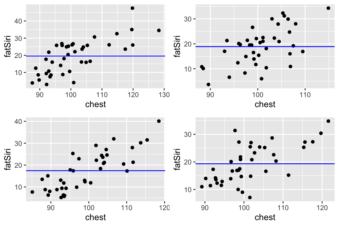
Ideally, both bias and variance would be low. BUT when we improve one of the features, we hurt the other. For example, consider two possible models of fatSiri: fatSiri ~ 1 (a model with only an intercept term & no predictors) and fatSiri ~ poly(chest, 7). Check out the behavior of the simpler fatSiri ~ 1 model across 4 different samples of 40 adults each:
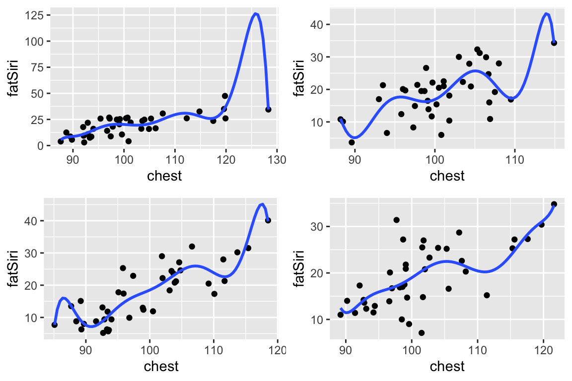
Similarly, check out the behavior of the more complicated fatSiri ~ poly(chest,7) model across these 4 different samples:
These 2 models illustrate the extremes:
The simpler model (
fatSiri ~ 1) has high bias (it doesn’t explain much aboutfatSiri) but low variability (it doesn’t vary much from sample to sample). Thus this model provides stability, but at the cost of not much info aboutfatSiri. It is too rigid.The complicated model (
fatSiri ~ poly(chest, 7)) has low bias (each of the models captures more detail infatSiri) but high variability (it varies a lot from sample to sample). Thus this model provides more detailed info aboutfatSiri, but at the cost of not being broadly generalizable beyond the sample at hand. It is too flexible / wiggly.
The goal in model building is to be in between these two extremes!
- LASSO and the bias-variance trade-off
Think back to the LASSO model above which depended upon tuning parameter \(\lambda\).- For which values of \(\lambda\) (small or large) will LASSO be the most biased?
- For which values of \(\lambda\) (small or large) will LASSO be the most variable?
- The Bias-Variance trade-off also comes into play when comparing across methods. Consider LASSO vs least squares:
- Which will tend to be more biased?
- Which will tend to be more variable?
- When will LASSO beat least squares in the bias-variance trade-off game?
12.4 HW2 solutions
Don’t peak unless and until you really, really need to!
Minnesota
Birthdays %>% filter(state == "MN", year == 1980) %>% arrange(desc(births)) %>% head() ## state year month day date wday births ## 1 MN 1980 12 19 1980-12-19 Fri 251 ## 2 MN 1980 9 3 1980-09-03 Wed 238 ## 3 MN 1980 6 19 1980-06-19 Thurs 237 ## 4 MN 1980 9 19 1980-09-19 Fri 234 ## 5 MN 1980 8 19 1980-08-19 Tues 233 ## 6 MN 1980 4 22 1980-04-22 Tues 231
Averaging births
Birthdays %>% summarize(mean(births)) ## mean(births) ## 1 189.0409 Birthdays %>% group_by(year) %>% summarize(mean(births)) ## # A tibble: 20 x 2 ## year `mean(births)` ## <int> <dbl> ## 1 1969 192. ## 2 1970 200. ## 3 1971 191. ## 4 1972 175. ## 5 1973 169. ## 6 1974 170. ## 7 1975 169. ## 8 1976 170. ## 9 1977 179. ## 10 1978 179. ## 11 1979 188. ## 12 1980 194. ## 13 1981 195. ## 14 1982 198. ## 15 1983 196. ## 16 1984 197. ## 17 1985 202. ## 18 1986 202. ## 19 1987 205. ## 20 1988 210. Birthdays %>% group_by(year, state) %>% summarize(mean(births)) %>% head() ## # A tibble: 6 x 3 ## # Groups: year [1] ## year state `mean(births)` ## <int> <chr> <dbl> ## 1 1969 AK 18.6 ## 2 1969 AL 174. ## 3 1969 AR 91.3 ## 4 1969 AZ 93.3 ## 5 1969 CA 954. ## 6 1969 CO 110.
Dates
Seasonality
Sleuthing
# a births_80_81 <- daily_births %>% filter(year %in% c(1980, 1981)) # b ggplot(births_80_81, aes(x = date, y = total, color = weekday)) + geom_point()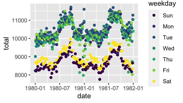
Superstition
friday_only <- daily_births %>% filter(weekday == "Fri") %>% mutate(fri_13 = (mday == 13)) ggplot(friday_only, aes(x = total, fill = fri_13)) + geom_density(alpha = 0.5)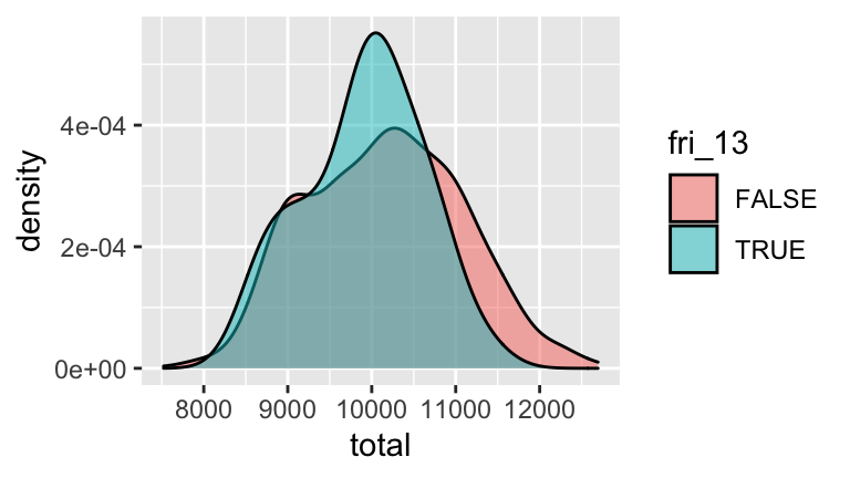
Best subset selection
# b 2^11 ## [1] 2048 # c library(leaps) best_subsets <- regsubsets(fatSiri ~ ., body_data, nvmax = 11) # Store the summary information best_summary <- summary(best_subsets) best_summary ## Subset selection object ## Call: regsubsets.formula(fatSiri ~ ., body_data, nvmax = 11) ## 11 Variables (and intercept) ## Forced in Forced out ## age FALSE FALSE ## weight FALSE FALSE ## height FALSE FALSE ## chest FALSE FALSE ## abdomen FALSE FALSE ## hip FALSE FALSE ## thigh FALSE FALSE ## knee FALSE FALSE ## ankle FALSE FALSE ## biceps FALSE FALSE ## wrist FALSE FALSE ## 1 subsets of each size up to 11 ## Selection Algorithm: exhaustive ## age weight height chest abdomen hip thigh knee ankle biceps wrist ## 1 ( 1 ) " " " " " " " " "*" " " " " " " " " " " " " ## 2 ( 1 ) " " " " "*" " " "*" " " " " " " " " " " " " ## 3 ( 1 ) " " " " "*" "*" "*" " " " " " " " " " " " " ## 4 ( 1 ) " " " " "*" "*" "*" " " " " " " " " "*" " " ## 5 ( 1 ) " " " " "*" "*" "*" " " " " "*" " " "*" " " ## 6 ( 1 ) " " "*" "*" "*" "*" " " " " "*" " " "*" " " ## 7 ( 1 ) " " "*" "*" "*" "*" "*" " " "*" " " "*" " " ## 8 ( 1 ) " " "*" "*" "*" "*" "*" " " "*" " " "*" "*" ## 9 ( 1 ) " " "*" "*" "*" "*" "*" " " "*" "*" "*" "*" ## 10 ( 1 ) "*" "*" "*" "*" "*" "*" " " "*" "*" "*" "*" ## 11 ( 1 ) "*" "*" "*" "*" "*" "*" "*" "*" "*" "*" "*"
Interpreting
# R^2 values for each model best_summary$rsq ## [1] 0.7019160 0.7220286 0.7510430 0.7799489 0.7864073 0.7877317 0.7907425 ## [8] 0.7908643 0.7908919 0.7908971 0.7908991 # R^2 value for the model with 5 predictors best_summary$rsq[5] ## [1] 0.7864073 # Coefficients of the model with 5 predictors) coef(best_subsets, 5) ## (Intercept) height chest abdomen knee biceps ## 24.6688609 -0.8707637 -0.5722038 1.1733167 -0.5548454 0.8083306 # b best_rsq <- data.frame(subset_size = c(1:11), rsq = best_summary$rsq) ggplot(best_rsq, aes(x = subset_size, y = rsq)) + geom_point() + geom_line()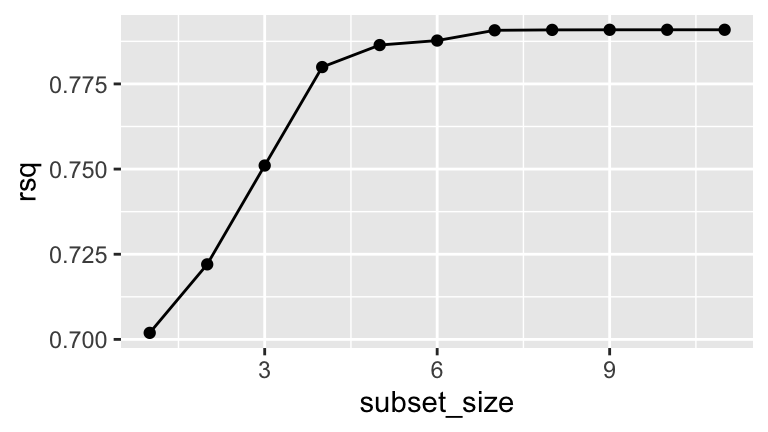
# c # This model has fairly high R^2. Though R^2 increases when we add more than 4 predictors, it's not enough to offset the added complexity. # d # Weight is likely multicollinear, or correlated, with the predictors here. Thus including it would be redundant. coef(best_subsets, 4) ## (Intercept) height chest abdomen biceps ## 25.6943547 -1.0075444 -0.6065834 1.1016493 0.7218723 # e # it's computationally expensive!! We had to fit more than 2000 models
- Shrinkage video
Run the LASSO
# Set the seed set.seed(2020) # Perform LASSO lasso_model <- train( fatSiri ~ ., data = body_data, method = "glmnet", trControl = trainControl(method = "cv", number = 10), tuneGrid = data.frame(alpha = 1, lambda = 10^seq(-3, 1, length = 100)), metric = "MAE" ) # a # the method and tuneGrid lines # b summary(10^seq(-3, 1, length = 100)) ## Min. 1st Qu. Median Mean 3rd Qu. Max. ## 0.00100 0.01001 0.10011 1.12555 1.00082 10.00000 # c # 10 predictors. Their coefs are closer to 0. coef(lasso_model$finalModel, 0.001) ## 12 x 1 sparse Matrix of class "dgCMatrix" ## 1 ## (Intercept) 60.605927304 ## age . ## weight 0.108468975 ## height -1.125039371 ## chest -0.709060303 ## abdomen 1.182836240 ## hip -0.205132525 ## thigh 0.017109987 ## knee -0.682776419 ## ankle 0.004328879 ## biceps 0.705024866 ## wrist 0.166699852 # d combined for ease of comparison (you can certainly print these separately) cbind(coef(lasso_model$finalModel, 0.001), coef(lasso_model$finalModel, 0.1), coef(lasso_model$finalModel, 1), coef(lasso_model$finalModel, 10)) ## 12 x 4 sparse Matrix of class "dgCMatrix" ## 1 1 1 1 ## (Intercept) 60.605927304 8.472577e+00 -35.14307208 20.4025 ## age . 8.565586e-05 . . ## weight 0.108468975 . . . ## height -1.125039371 -7.035691e-01 . . ## chest -0.709060303 -3.974397e-01 . . ## abdomen 1.182836240 9.979675e-01 0.56420517 . ## hip -0.205132525 . . . ## thigh 0.017109987 . . . ## knee -0.682776419 -3.130690e-01 . . ## ankle 0.004328879 . . . ## biceps 0.705024866 6.167842e-01 0.07564217 . ## wrist 0.166699852 . . .```
Visualizing LASSO
# Plot coefficients for each LASSO
plot(lasso_model$finalModel, xvar = "lambda", label = TRUE, col = rainbow(20))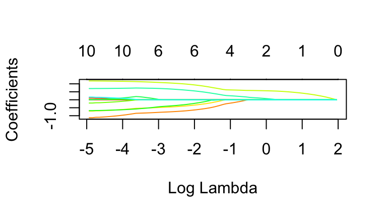
- plot: examining coefficients
- The y-intercepts are roughly equivalent to the least squares coefficients.
- Yep.
- plot: examining predictors
- biceps
- roughly 0.25
- answers will vary. roughly \(\log(\lambda) \approx -2\)
- \(\log(\lambda) \approx 0.25\)
- biceps
- big picture
- The predictor coef lines shrink to 0 as \(\lambda\) increases.
- abdomen (variable 5)
- weight (2), hip (6), and others
- 4
tuning
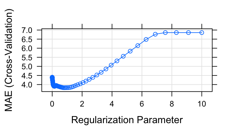
# a
# When lambda is too small, the model contains too many predictors thus is overfit to the sample data (thus has high CV MAE).
# When lambda is too big, the model contains too few predictors, thus doesn't contain useful info about fatSiri (thus CV MAE is high)

# b
# 0.5ish

# c
lasso_model$bestTune$lambda
## [1] 0.8111308
Examining the best LASSO
# a
coef(lasso_model$finalModel, lasso_model$bestTune$lambda)

# b (two approaches)
lasso_model$resample %>%
  summarize(mean(MAE))
lasso_model$results %>%
  filter(lambda == lasso_model$bestTune$lambda)

# c
# Though their CV MAE are similar, I'd choose the LASSO since it's so much simpler (with only 2 predictors) than the LM (with 11 predictors).
- LASSO and the bias-variance trade-off
- large. As \(\lambda\) increase, the model has fewer predictors and will be more rigid.
- small. When \(\lambda\) is small, the model will include all / most predictors thus might be overfit to our sample (and vary a lot from sample to sample).
- The Bias-Variance trade-off also comes into play when comparing across methods. Consider LASSO vs least squares:
- Which will tend to be more biased? LASSO (it tends to be more rigid)
- Which will tend to be more variable? LM
- When will LASSO beat least squares in the bias-variance trade-off game? When using all predictors causes overfitting (generally when we have a lot of predictors relative to a smaller sample size)