10 Building models
Announcements
Homework 3 is due today. The 5-day extension goes to Sunday at 9:30am. Flexibility has trade-offs, thus you’re strongly encouraged to only use the extension when absolutely necessary. Submitting homework by the deadline will ensure that you’re practicing concepts on the same timeline that we’re discussing them, prepare you for the next material, and make the workload pacing more manageable.
Quiz 1 is on Thursday. Please see details on page 7 of the syllabus. I recommend that you review each activity and homework, trying to answer the questions without first looking at your notes.
10.1 Getting started
REVIEW: COVARIATES
# Load packages & data
library(ggplot2)
library(dplyr)
CPS_2018 <- read.csv("https://www.macalester.edu/~ajohns24/data/CPS_2018.csv")

# We'll focus on 18 to 34-year-olds that make under 250,000 dollars
CPS_2018 <- CPS_2018 %>%
  filter(age >= 18, age <= 34) %>%
  filter(wage < 250000) %>%
    mutate(age_months = age*12)

# Model 1
CPS_model_1 <- lm(wage ~ marital, CPS_2018)
coef(summary(CPS_model_1))
##                Estimate Std. Error   t value     Pr(>|t|)
## (Intercept)    46145.23    921.062  50.10002 0.000000e+00
## maritalsingle -17052.37   1127.177 -15.12839 5.636068e-50

# Model 4
CPS_model_4 <- lm(wage ~ marital + age + education + industry, CPS_2018)
coef(summary(CPS_model_4))
##                                   Estimate Std. Error    t value     Pr(>|t|)
## (Intercept)                     -52498.857  7143.8481 -7.3488206 2.533275e-13
## maritalsingle                    -5892.842  1105.6898 -5.3295615 1.053631e-07
## age                               1493.360   116.1673 12.8552586 6.651441e-37
## education                         3911.117   243.0192 16.0938565 4.500408e-56
## industryconstruction              5659.082  6218.5649  0.9100302 3.628760e-01
## industryinstallation_production   1865.650  6109.2613  0.3053806 7.600964e-01
## industrymanagement                1476.884  6031.2901  0.2448704 8.065727e-01
## industryservice                  -7930.403  5945.6509 -1.3338158 1.823603e-01
## industrytransportation           -1084.176  6197.2462 -0.1749448 8.611342e-01
Interpret the
maritalcoefficient in both models.Interpret the
industrytransportationcoefficient inCPS_model_4.If we had to draw the model, it would look like 12 parallel planes. Which combo of marital status and industry are represented by the top plane? The bottom plane?
WHERE ARE WE
There are 3 important steps in statistical modeling:
- building some models
- interpreting the models
- evaluating the models
Today we’ll talk more about model building. This can be an overwhelming task – there are countless options! Here are some things that can make the process less overwhelming:
Model building should be guided by our research questions and goals. These can vary:
- Sometimes we’re interested in a specific set of variables, thus should use these variables in our model.
- Sometimes we’re less interested in a specific set of variables. Instead, we might be interested in:
- building a strong model, i.e. one that will give us good predictions
- building a parsimonious model, i.e. one that will give us good predictions while still being relatively simple.
- building a strong model, i.e. one that will give us good predictions
There’s typically not one “best” model, but countless reasonable models.
Rarely would we build just one model. Rather, a set of models can provide a more complete picture of our research questions.
It’s important to start small (eg: with 1 predictor) and build up from there.
10.2 Exercises
10.2.1 Part 1
Consider 5 models of wages:
| Model | Predictors | R2 |
|---|---|---|
CPS_model_1 |
marital | 0.067 |
CPS_model_2 |
marital, age | 0.157 |
CPS_model_3 |
marital, age, education | 0.257 |
CPS_model_4 |
marital, age, education, industry | 0.280 |
CPS_model_5 |
marital, age, education, industry, hours, health | 0.341 |
- A set of models
For what research goal would models 1 and 5 be a good set of models to present?
- Strength
Which is the best model if we want the strongest model of wages and don’t care how complex it is?
- Parsimony
Which is the best model if we want a parsimonious model, i.e. we want to maximize our understanding of why wages vary from person to person while keeping our model as simple as possible?
- Strength vs parsimony
In which of the following cases would a parsimonious model likely be a goal:- A local nonprofit asks you to develop a model that they can use to track donations throughout the year.
- Netflix asks you to develop a model that is good at recommending movies to its users.
- A local nonprofit asks you to develop a model that they can use to track donations throughout the year.
- Redundancy & multicollinearity
Take a quick peak at some R-squared values for 4 different models of wage:Why are the R-squared values for models a and b the same? NOTE:
age_months=age * 12# model a summary(lm(wage ~ age, CPS_2018))$r.squared ## [1] 0.1463378 # model b summary(lm(wage ~ age_months + age, CPS_2018))$r.squared ## [1] 0.1463378How does the R-squared for model c compare to that of models a and b? Why isn’t it bigger, eg: closer to the sum of the R-squared values from models a and b?
# model a
summary(lm(wage ~ age, CPS_2018))$r.squared
## [1] 0.1463378

# model b
summary(lm(wage ~ marital, CPS_2018))$r.squared
## [1] 0.06739606

# model c
summary(lm(wage ~ age + marital, CPS_2018))$r.squared
## [1] 0.1568834
10.2.2 Part 2
In Part 2, let’s dive deeper into important considerations when building a strong model. We’ll use the following data on penguins:
# Load data on penguins.
library(palmerpenguins)
data(penguins)

# For illustration purposes only, take a sample of 10 penguins.
# We'll discuss this code later in the course!
set.seed(155)
penguins_small <- sample_n(penguins, size = 10) %>%
  mutate(flipper_length_mm = jitter(flipper_length_mm))
Consider 3 models of bill length:
# A model with one predictor (flipper_length_mm)
poly_mod_1 <- lm(bill_length_mm ~ flipper_length_mm, penguins_small)

# A model with two predictors (flipper_length_mm and flipper_length_mm^2)
poly_mod_2 <- lm(bill_length_mm ~ poly(flipper_length_mm, 2), penguins_small)

# A model with nine predictors (flipper_length_mm, flipper_length_mm^2, ... on up to flipper_length_mm^9)
poly_mod_9 <- lm(bill_length_mm ~ poly(flipper_length_mm, 9), penguins_small)
- What’s best? Using your gut.
Before doing any analysis, which of the three models do you think will be best? Post your answer to this anonymous survey.
What’s best? Using R-squared.
Calculate the R-squared values of these 3 models. Which model do you think is best?summary(poly_mod_1)$r.squared ## [1] 0.7341412 summary(poly_mod_2)$r.squared ## [1] 0.7630516 summary(poly_mod_9)$r.squared ## [1] 1
What’s best? Using visualization & context.
Check out plots of these 3 models. Which model do you think is best? Post your answer to this anonymous survey.# A plot of model 1 ggplot(penguins_small, aes(y = bill_length_mm, x = flipper_length_mm)) + geom_point() + geom_smooth(method = "lm", se = FALSE) # A plot of model 2 ggplot(penguins_small, aes(y = bill_length_mm, x = flipper_length_mm)) + geom_point() + geom_smooth(method = "lm", formula = y ~ poly(x, 2), se = FALSE) # A plot of model 9 ggplot(penguins_small, aes(y = bill_length_mm, x = flipper_length_mm)) + geom_point() + geom_smooth(method = "lm", formula = y ~ poly(x, 9), se = FALSE)
- Cooking
- List 3 of your favorite foods.
- Now imagine making a dish that combines all of these foods. Do you think it would taste good?
- List 3 of your favorite foods.
- Too many good things doesn’t make a better thing
Model 9 demonstrates that it’s always possible to get a perfect R-squared of 1, but there are drawbacks to putting more and more predictors into our model. Answer the following about model 9:- How easy would it be to interpret this model?
- Would you say that this model captures the general trend of the relationship between
bill_length_mmandflipper_length_mm?
- How well do you think this model would generalize to penguins that were not included in the
penguins_smallsample? For example, would you expect these new penguins to fall on the wiggly model 9 curve?
- How easy would it be to interpret this model?
Overfitting
Model 9 provides an example of a model that’s overfit to our sample data. That is, it’s built to pick up the tiny details of our data at the cost of losing the more general trends of the relationship of interest. Check out the image from the front page of the manual. Which plot pokes fun at overfitting?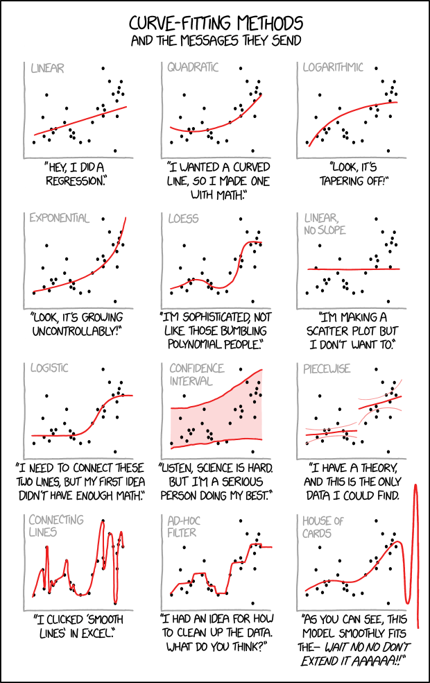
Some other goodies:


- Questioning R-squared
Zooming out, explain some limitations of relying on R-squared to measure the strength / usefulness of a model.
OPTIONAL: Beyond R^2
We’ve seen that, unless a predictor is redundant with another, R-squared will increase. Even if that predictor is strongly multicollinear with another. Even if that predictor isn’t a good predictor! Thus if we only look at R-squared we might get overly greedy. We can check our greedy impulses a few ways. We take a more in depth approach in STAT 253, but one quick alternative is reported right in our modelsummary()tables. Adjusted R-squared includes a penalty for incorporating more and more predictors. Mathematically:\[\text{Adj R^2} = R^2 - (1-R^2)\frac{\text{number of non-intercept coefficients}}{\text{sample size}} = R^2 - \text{ penalty}\]
Thus unlike R-squared, Adjusted R-squared can decrease when the information that a predictor contributes to a model isn’t enough to offset the complexity it adds to that model. Consider two models:
example_1 <- lm(bill_length_mm ~ species, penguins) example_2 <- lm(bill_length_mm ~ species + island, penguins)- Check out the summaries for the 2 example models. In general, how does a model’s Adjusted R-squared compare to the R-squared? Is it greater, less than, or equal to the R-squared?
- How did the R-squared change from example model 1 to model 2? How did the Adjusted R-squared change?
- Explain what it is about
islandthat resulted in a decreased Adjusted R-squared. Note: it’s not necessarily the case thatislandis a bad predictor on its own!
10.3 Solutions
- A set of models These would help us understand the overall wage gap for single vs married people and how much of these can be explained by the covariates.
- Strength Model 5 has the highest R-squared.
- Parsimony Model 3 or 4 – their R-squareds are nearly as high as that for Model 5, but have fewer predictors.
- Strength vs parsimony
- A parsimonious model would be simpler to understand and implement.
- So long as the model gave good recommendations, a parsimonious model wouldn’t be necessary.
- Redundancy & multicollinearity
- The predictors are redundant – they have the same exact info, just on different scales.
- Age and marital status are multicollinear, thus including both won’t drastically improve the R-squared in comparison to using just age alone.
- What’s best? Using your gut. Answers will vary.
- What’s best? Using R-squared. Answers will vary.
8.What’s best? Using visualization & context. Answers will vary.
```r
# A plot of model 1
g1 <- ggplot(penguins_small, aes(y = bill_length_mm, x = flipper_length_mm)) +
  geom_point() +
  geom_smooth(method = "lm", se = FALSE)

# A plot of model 2
g2 <- ggplot(penguins_small, aes(y = bill_length_mm, x = flipper_length_mm)) +
  geom_point() +
  geom_smooth(method = "lm", formula = y ~ poly(x, 2), se = FALSE)

# A plot of model 9
g3 <- ggplot(penguins_small, aes(y = bill_length_mm, x = flipper_length_mm)) +
  geom_point() +
  geom_smooth(method = "lm", formula = y ~ poly(x, 9), se = FALSE)

grid.arrange(g1, g2, g3, ncol = 3)
```

<img src="155_S2022_manual_files/figure-html/unnamed-chunk-232-1.png" width="768" style="display: block; margin: auto;" />
- Cooking
- Will vary.
- Gross.
- Too many good things doesn’t make a better thing
- NOT easy to interpret.
- NO. It’s much more wiggly than the general trend.
- NOT WELL. It is too tailored to our data.
- Overfitting The bottom left plot.
- Questioning R-squared It measures how well our model explains / predicts our sample data, not how well it explains / predicts the broader population.
OPTIONAL: Beyond R^2
example_1 <- lm(bill_length_mm ~ species, penguins) example_2 <- lm(bill_length_mm ~ species + island, penguins)- It’s less than the R-squared
- R-squared increased and Adjusted R-squared decreased.
- It didn’t provide “significant” information about bill length beyond what was already provided by species.