19 Using confidence intervals for testing hypotheses
Announcements
- Checkpoint 16 is due Tuesday. The video is 17ish minutes. This is an important one to not miss!
- Mini-project phase 1 is due Tuesday.
- I want to hear from more people today! I will assign each table an example to discuss with the class.
19.1 Getting started
Today’s goal
We’ve used confidence intervals to communicate the error in our sample estimates and provide a range of plausible values for the population features we’re estimating. Next, we’ll:
- Use confidence intervals to test hypotheses about the population.
- Construct confidence and prediction intervals for the outcomes of our response variable.
The data story
Using the high_peaks data on hiking trails in the Adirondack mountains of northern New York state, we’ll explore whether the time it takes to complete each hike is associated with various features: a hike’s highest elevation, length, ascent, and difficulty rating.
# Load packages
library(ggplot2)
library(dplyr)

# Import data
peaks <- read.csv("https://www.macalester.edu/~ajohns24/data/high_peaks.csv")
EXAMPLE 1
Consider the relationship between y, the time it takes to complete a hike (in hours), by x, its highest elevation (in feet):
\[y = \beta_0 + \beta_1 x\]
Since we don’t have data on all hikes, we can’t know what this model is. But we can estimate it using our sample data:
model_1 <- lm(time ~ elevation, peaks)
coef(summary(model_1))
##                  Estimate  Std. Error    t value  Pr(>|t|)
## (Intercept) 11.2113764116 5.195379956  2.1579512 0.0364302
## elevation   -0.0001269391 0.001175554 -0.1079824 0.9145006
Use the 68-95-99.7 Rule along with information from the model table to calculate an approximate 95% CI for \(\beta_1\), the actual elevation coefficient.
Then check your work:
confint(model_1, level = 0.95)
##                    2.5 %       97.5 %
## (Intercept)  0.740776111 21.681976712
## elevation   -0.002496112  0.002242234
EXAMPLE 2
What can we conclude from the 95% CI for \(\beta_1\)?
- Our sample data establishes a significant negative association between hiking time and elevation.
- Our sample data establishes a significant positive association between hiking time and elevation.
- Our sample data does not establish a significant association between hiking time and elevation.
- Our sample data establishes a significant negative association between hiking time and elevation.
Alternatively (yet equivalently), answer this question using the confidence bands around our sample model trend. NOTE: These confidence bands are reminiscent of our sampling distribution simulations which produced a range of model trends.
ggplot(peaks, aes(x = elevation, y = time)) +
  geom_point() +
  geom_smooth(method = "lm")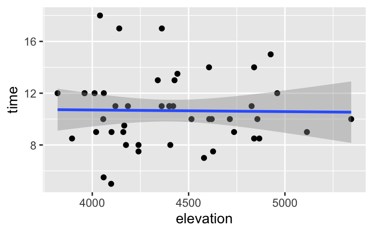
EXAMPLE 3
Next, let’s use our data to make inferences about the relationship between the time it takes to complete a hike in hours (y), by the hike’s vertical ascent, or the total change in elevation in feet (x):
model_2 <- lm(time ~ ascent, peaks)
coef(summary(model_2))
##                Estimate   Std. Error  t value    Pr(>|t|)
## (Intercept) 4.210054144 1.8661683434 2.255988 0.029092788
## ascent      0.002080525 0.0005908537 3.521218 0.001013549
A 95% CI for the actual ascent coefficient ranges from 0.0009 to 0.003:
confint(model_2, level = 0.95)
##                    2.5 %      97.5 %
## (Intercept) 0.4490389766 7.971069312
## ascent      0.0008897376 0.003271313
How can we interpret this CI?
We’re 95% confident that for every 1 foot increase in ascent, the completion time for all hikes in the population typically increases by somewhere between 0.0009 and 0.003 hours. (Or, increases somewhere between 0.9 and 3 hours for every 1000 foot increase in ascent.)
We’re 95% confident that for every 1 foot increase in ascent, the completion time for all hikes in our sample typically increases by somewhere between 0.0009 and 0.003 hours. (Or, increases somewhere between 0.9 and 3 hours for every 1000 foot increase in ascent.)
For 95% of all hikes, completion time will increase peaks size will increase by somewhere between 0.0009 and 0.003 hours for every extra 1 foot increase in ascent.
EXAMPLE 4
What can we conclude from the 95% CI for \(\beta_1\)?
- Our sample data establishes a significant negative association between hiking time and ascent.
- Our sample data establishes a significant positive association between hiking time and ascent.
- Our sample data does not establish a significant association between hiking time and ascent.
- Our sample data establishes a significant negative association between hiking time and ascent.
Alternatively (yet equivalently), answer this question using the confidence bands around our sample model trend.
ggplot(peaks, aes(x = ascent, y = time)) +
  geom_point() +
  geom_smooth(method = "lm")
EXAMPLE 5
In the previous example, we concluded that there’s a statistically significant association between hiking time and ascent. This means that an association exists. It does not necessarily mean that the association is meaningful, i.e. practically significant (as much as people mistakenly assume).
It’s important to follow up a technical confidence interval with some context. To this end, do you think that the association between hiking time and ascent is also practically significant? Mainly, in the context of hiking, is the magnitude of the association (i.e. an increase between 0.9 and 3 hours for every 1000 foot increase in ascent) actually meaningful?
EXAMPLE 6
Next let’s estimate the relationship between the time it takes to complete a hike, by the hike’s ascent and its length (in miles):
model_3 <- lm(time ~ ascent + length, peaks)
coef(summary(model_3))
##                 Estimate   Std. Error   t value     Pr(>|t|)
## (Intercept) 1.4383697458 1.1285627199 1.2745147 2.093258e-01
## ascent      0.0003047436 0.0003940533 0.7733563 4.435424e-01
## length      0.6577267333 0.0707823643 9.2922402 7.632252e-12
A 95% CI for the actual ascent coefficient ranges from -0.0005 to 0.0011:
confint(model_3, level = 0.95)
##                     2.5 %      97.5 %
## (Intercept) -0.8375938879 3.714333379
## ascent      -0.0004899406 0.001099428
## length       0.5149804913 0.800472975
What can we conclude from the 95% CI?
- Hiking time and ascent are significantly associated.
- Hiking time and ascent are not significantly associated (i.e. ascent is not a significant predictor of hiking time).
- When controlling for hike length, hiking time and ascent are significantly associated.
- When controlling for hike length, hiking time and ascent are not significantly associated (i.e. ascent is not a significant predictor of hiking time).
EXAMPLE 7
When considered alone in model_2, vertical ascent was a significant predictor of hiking time. Yet when considered along with hike length in model_3, it wasn’t. Explain why this happened. Better yet, support your explanation with some new graphical or numerical evidence.
EXAMPLE 8
Reconsider model_3. If we already have vertical ascent in our model, is hike length a significant / useful predictor of hiking time? Why or why not?
19.2 Exercises
Goal
Use confidence interval techniques to communicate and understand the uncertainty in predictions made from our sample models.
Model prediction
Consider a model of hiking time (in hours) vs length (in miles):model_4 <- lm(time ~ length, peaks) coef(summary(model_4)) ## Estimate Std. Error t value Pr(>|t|) ## (Intercept) 2.0481729 0.80370575 2.548411 1.438759e-02 ## length 0.6842739 0.06161802 11.105095 2.390128e-14There are 2 types of predictions we can make for, say, a hiking length of 10 miles:
- Predict the average hiking time for all 10-mile hikes in the world.
- Predict the hiking time for the “Minnesota trail”, a specific 10-mile hike.
The values of the two predictions are the same:
time = 2.0482 + 0.6843*10 = 8.89 hoursHowever, the potential error in these predictions differs. Check in with your intuition: Is there more error in trying to predict the average hiking time of all 10-mile hikes in the world, or the exact hiking time of the Minnesota trail, a specific 10-mile hike? Explain your reasoning.
- Confidence intervals & confidence bands
Check your intuition. Calculate and report the 95% confidence interval for the average hiking time of all 10-mile hikes:
predict(model_4,
        newdata = data.frame(length = 10),
        interval = "confidence", level = 0.95)
NOTE:
fitis the prediction (which due to rounding is slightly different than our “by hand” prediction),lwrgives the lower bound of the CI, anduprgives the upper bound of the CI.What’s the best interpretation of this interval?
- Among the 10-mile long hikes in our sample, we’re 95% confident that the average hiking time is in this interval.
- Among all 10-mile long hikes in the world, we’re 95% confident that the average hiking time is in this interval.
- We’re 95% confident that the hiking time for the Minnesota trail is in this interval.
- Among the 10-mile long hikes in our sample, we’re 95% confident that the average hiking time is in this interval.
We can visualize the confidence interval for the average hiking length of all hikes at any common length (not just 10 miles) by drawing confidence bands around the model. The vertical line drawn at a length of 10 miles reflects the interval you calculated above. NOTE: What have we changed in the syntax?
ggplot(peaks, aes(x = length, y = time)) +
  geom_point() +
  geom_smooth(method = "lm") +
  geom_segment(aes(x = 10, xend = 10, y = 8.354608, yend = 9.427217), color = "red")
- Prediction intervals
Calculate and report the 95% prediction interval (PI) for the hiking time for the Minnesota trail, a specific 10-mile hike. NOTE: What changed in the syntax?
predict(model_4,
        newdata = data.frame(length = 10),
        interval = "prediction", level = 0.95)
How can we interpret this interval?
- Among the 10-mile long hikes in our sample, we’re 95% confident that the average hiking time is in this interval.
- Among all 10-mile long hikes in the world, we’re 95% confident that the average hiking time is in this interval.
- We’re 95% confident that the hiking time for the Minnesota trail is in this interval.
- Among the 10-mile long hikes in our sample, we’re 95% confident that the average hiking time is in this interval.
Prediction vs confidence bands
We can visualize the prediction interval for the hiking time of a trail at any length by drawing prediction bands. This requires some messy syntax:# Calculate and store prediction intervals for every length value predictions_1 <- data.frame(peaks, predict(model_4, newdata = data.frame(length = peaks$length), interval = 'prediction')) # Check it out head(predictions_1)# Plot regression line with prediction bands ggplot(predictions_1, aes(x = length, y = time)) + geom_point() + geom_smooth(method = 'lm', color = "blue") + geom_ribbon(aes(y = fit, ymin = lwr, ymax = upr, fill = 'prediction'), alpha = 0.2)- Do the confidence bands (darker gray) capture our uncertainty about the hiking time for the AVERAGE HIKE or for INDIVIDUAL / SPECIFIC HIKES?
- Do the prediction bands (lighter gray) capture our uncertainty about the hiking time for the AVERAGE HIKE or for INDIVIDUAL / SPECIFIC HIKES?
- Which are wider, intervals for the average hiking time for all hikes of a common length OR intervals for the exact hiking time for a specific, individual hike at that length? Explain why this makes intuitive sense.
- Do the confidence bands (darker gray) capture our uncertainty about the hiking time for the AVERAGE HIKE or for INDIVIDUAL / SPECIFIC HIKES?
- Narrowing
Though it’s not as noticeable with the prediction bands, these and the confidence bands are always the most narrow at the same point – in this case at a length of 12.57391 miles. What other meaning does this value have? Provide some proof and explain why it makes intuitive sense that the bands are narrowest at this point.
Extra practice
Reconsider the model of hiking time versus ascent,model_2.- Construct and interpret a 95% prediction interval for the hiking time for the Minnesota Trail, which has a vertical ascent of 1800 feet.
- Construct and interpret a 95% confidence interval for the average hiking time among all hikes that have an 1800-foot vertical ascent.
19.3 Solutions
EXAMPLE 1
-0.0001269391 - 2*0.001175554
## [1] -0.002478047
-0.0001269391 + 2*0.001175554
## [1] 0.002224169
confint(model_1, level = 0.95)
## 2.5 % 97.5 %
## (Intercept) 0.740776111 21.681976712
## elevation -0.002496112 0.002242234
EXAMPLE 2
Our sample data does not establish a significant association between hiking time and elevation.
The bands include 0-slope lines
EXAMPLE 3
- We’re 95% confident that for every 1 foot increase in ascent, the completion time for all hikes in the population typically increases by somewhere between 0.0009 and 0.003 hours. (Or, increases somewhere between 0.9 and 3 hours for every 1000 foot increase in ascent.)
EXAMPLE 4
Our sample data establishes a significant positive association between hiking time and ascent.
The bands do not include any 0-slope lines.
EXAMPLE 5
I think so.
EXAMPLE 6
When controlling for hike length, hiking time and ascent are not significantly associated (i.e. ascent is not a significant predictor of hiking time).
EXAMPLE 7
Multicollinearity. When length isn’t in the model, vertical ascent is a significant predictor of hiking time. Yet hikes with greater ascent also tend to be longer (ascent and length are correlated). Thus if we already know a hike’s length, then its vertical ascent doesn’t provide a significant amount of additional information about hiking time.
EXAMPLE 8
Yes. It’s CI is entirely and meaningfully above 0.
- Model prediction
Your intuition will vary. Your intuition might be right or wrong, the important thing is to pause and reflect.
- Confidence intervals & confidence bands
.
predict(model_4, newdata = data.frame(length = 10), interval = "confidence", level = 0.95) ## fit lwr upr ## 1 8.890912 8.354608 9.427217Among all 10-mile long hikes in the world, we’re 95% confident that the average hiking time is in this interval.
.
ggplot(peaks, aes(x = length, y = time)) + geom_point() + geom_smooth(method = "lm") + geom_segment(aes(x = 10, xend = 10, y = 8.354608, yend = 9.427217), color = "red")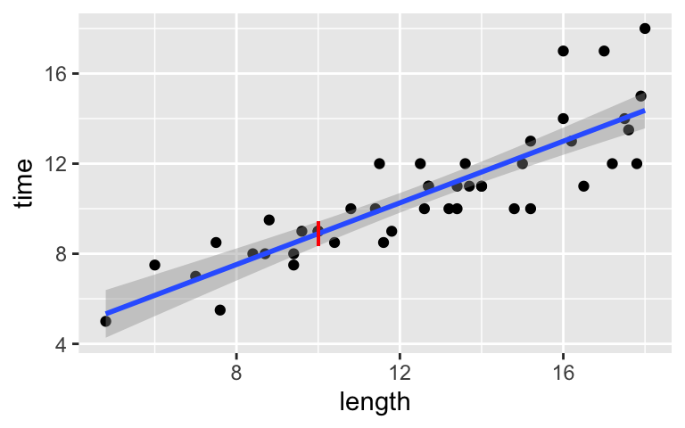
- Prediction intervals
NOTE: we changed
intervalto"prediction"predict(model_4, newdata = data.frame(length = 10), interval = "prediction", level = 0.95) ## fit lwr upr ## 1 8.890912 5.921304 11.86052We’re 95% confident that the hiking time for the Minnesota trail is in this interval.
Prediction vs confidence bands
# Calculate and store prediction intervals for every length value predictions_1 <- data.frame(peaks, predict(model_4, newdata = data.frame(length = peaks$length), interval = 'prediction')) # Check it out head(predictions_1) ## peak elevation difficulty ascent length time rating fit ## 1 Mt. Marcy 5344 5 3166 14.8 10.0 moderate 12.175427 ## 2 Algonquin Peak 5114 5 2936 9.6 9.0 moderate 8.617203 ## 3 Mt. Haystack 4960 7 3570 17.8 12.0 difficult 14.228249 ## 4 Mt. Skylight 4926 7 4265 17.9 15.0 difficult 14.296676 ## 5 Whiteface Mtn. 4867 4 2535 10.4 8.5 easy 9.164622 ## 6 Dix Mtn. 4857 5 2800 13.2 10.0 moderate 11.080589 ## lwr upr ## 1 9.210158 15.14070 ## 2 5.641838 11.59257 ## 3 11.205404 17.25109 ## 4 11.271141 17.32221 ## 5 6.199949 12.12929 ## 6 8.127210 14.03397# Plot regression line with prediction bands ggplot(predictions_1, aes(x = length, y = time)) + geom_point() + geom_smooth(method = 'lm', color = "blue") + geom_ribbon(aes(y = fit, ymin = lwr, ymax = upr, fill = 'prediction'), alpha = 0.2)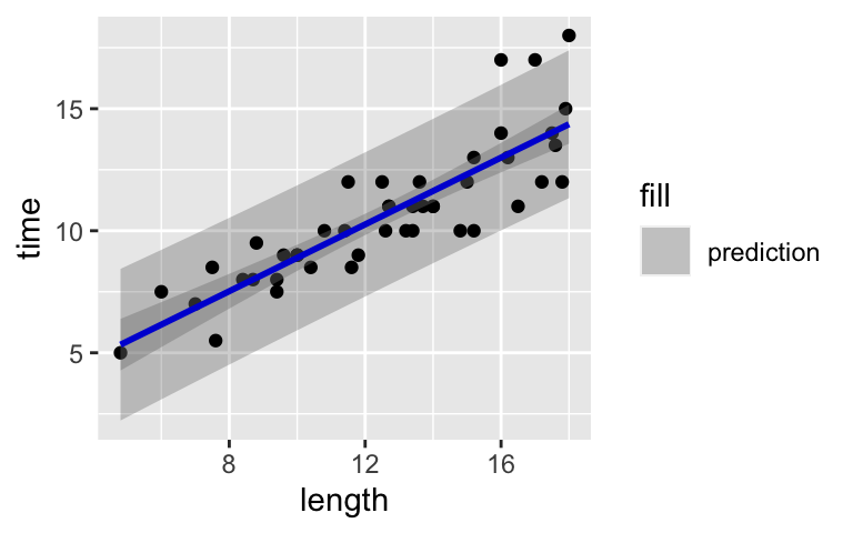
- average hike
- individual / specific hikes
- Intervals for the exact hiking time for a specific, individual hike are wider. It’s tougher to anticipate the exact behavior of an individual data point (it could be an outlier!), and easier to anticipate the average behavior of a group of data points (where any outliers are averaged out).
- average hike
- Narrowing
This is the average hiking length. Why’s there less error here? Conceptually, it’s easier to anticipate the hiking time (y) for hikes of the typical length. Further, there are more data points, hence information, in the middle here than at the extremes of hiking length.
Extra practice
# a
# We're 95% confident that it would take between
# 2.64 and 13.27 hours to complete this hike
predict(model_2,
        newdata = data.frame(ascent = 1800),
        interval = "prediction", level = 0.95)
##        fit      lwr      upr
## 1 7.954999 2.640613 13.26939

# b
# We're 95% confident that among all 10-mile hikes,
# the typical completion time is between 6.24 and 9.67 hours.
predict(model_2,
        newdata = data.frame(ascent = 1800),
        interval = "confidence", level = 0.95)
##        fit      lwr      upr
## 1 7.954999 6.242312 9.667686