21 Cautions in hypothesis testing – I
Announcements
- Today is the last day to hand in mini-project Phase 1 for credit.
- Homework 7 (last homework!) & Mini-project Phase 2 are due one week from today, on Thursday, April 21. There will be class time to work on these today and all next week. Please use this time to minimize stress outside class!
- Homework 7 is longer than usual (hence why you’ll have so much class time to consider it). It is an important broad, though not exhaustive, review of the semester!
21.1 Getting started
The whole point
We can use sample data to estimate features of the population.
There’s error in this estimation.
Taking this error into account, we want to make some sort of conclusion about the population.
There is some gray area in this conclusion and we might be wrong. NOTE: This includes but is not limited to the chance of making a Type I or Type II error (not because we did anything wrong, but because we got unlucky data which led to an incorrect conclusion).
| . | \(H_0\) true | \(H_0\) not true |
|---|---|---|
| conclude results aren’t significant | Correct! | Type II Error (false negative) |
| conclude results are significant | Type I Error (false positive) | Correct! |
WARM-UP
What can we conclude about the association of mountain climber success with their age, their oxygen use, the height of their climb, and whether or not they did the hike solo (as opposed to in a team)? What type of errors might we be making?
# Load packages and data
library(dplyr)
library(ggplot2)
climbers <- read.csv("https://www.macalester.edu/~ajohns24/data/climbers_sub.csv")

# Build the model of success
climb_model <- glm(success ~ age + oxygen_used, climbers, family = "binomial")
coef(summary(climb_model))
##                    Estimate  Std. Error   z value      Pr(>|z|)
## (Intercept)     -0.51957247 0.207331212 -2.506002  1.221049e-02
## age             -0.02197407 0.005459778 -4.024718  5.704361e-05
## oxygen_usedTRUE  2.89559690 0.126370801 22.913496 3.408591e-116

# Check out the confidence intervals
confint(climb_model)
##                       2.5 %      97.5 %
## (Intercept)     -0.92682316 -0.11372877
## age             -0.03275496 -0.01134335
## oxygen_usedTRUE  2.65182522  3.14753145
exp(confint(climb_model))
##                      2.5 %     97.5 %
## (Intercept)      0.3958091  0.8925000
## age              0.9677757  0.9887207
## oxygen_usedTRUE 14.1798965 23.2785293
21.2 Exercises
Directions
- Explore common abuses of hypothesis testing so that (1) you don’t make these mistakes yourself; and (2) you can read others’ work with a healthy critical eye.
- Review. The exercises focus on new concepts, yet they require the understanding of “old” material. Though you won’t be required to do so, make sure you could write down model formulas, make predictions, interpret coefficients, etc if asked.
- Warm-up: gray area
Scroll down and check out the list in this article. Why is this funny?
The claim
Two researchers make a claim: songs in thelatingenre are longer than those in thepop/edmgenres. Thus they’re interested in the population model of songduration(in seconds) bylatin_genre:duration = \(\beta_0\) + \(\beta_1\) latin_genreTRUE
where population coefficients \(\beta_0\) and \(\beta_1\) are unknown. Which set of hypotheses align with the researchers’ claim?
- \(H_0\): \(\beta_1 = 0\) vs \(H_a\): \(\beta_1 < 0\)
- \(H_0\): \(\beta_1 = 0\) vs \(H_a\): \(\beta_1 \ne 0\)
- \(H_0\): \(\beta_1 = 0\) vs \(H_a\): \(\beta_1 > 0\)
- \(H_0\): \(\beta_1 = 0\) vs \(H_a\): \(\beta_1 < 0\)
Researcher 1
To test these hypotheses, Researcher 1 collects data on 20 songs and uses this to model songduration(in seconds) bylatin_genre:# Load the data spotify_small <- read.csv("https://www.macalester.edu/~ajohns24/data/spotify_example_small.csv") %>% select(track_artist, track_name, duration_ms, latin_genre) %>% mutate(duration = duration_ms / 1000) # Construct the model spotify_model_1 <- lm(duration ~ latin_genre, spotify_small) coef(summary(spotify_model_1)) ## Estimate Std. Error t value Pr(>|t|) ## (Intercept) 214.99869 12.97571 16.56932 2.412163e-12 ## latin_genreTRUE 39.45606 29.01458 1.35987 1.906619e-01Using the 68-95-99.7 Rule and
confint(), construct an approximate 95% confidence interval for the actuallatin_genrepopulation coefficient \(\beta_1\).Interpret your CI from part a.
Using this confidence interval alone, what conclusion do you make about the hypotheses?
- We have statistically significant evidence that latin genre songs tend to be longer than pop / edm songs.
- We do not have statistically significant evidence that latin genre songs tend to be longer than pop / edm songs.
- We have statistically significant evidence that latin genre songs tend to be longer than pop / edm songs.
Researcher 2 – part 1
Researcher 2 has the same research question, but gathers a different set of data:spotify_big <- read.csv("https://www.macalester.edu/~ajohns24/data/spotify_example_big.csv") %>% select(track_artist, track_name, duration_ms, latin_genre) %>% mutate(duration = duration_ms / 1000)- How many songs did Researcher 2 collect in
spotify_big? - Using the
spotify_bigdata, construct and comment on a visualization of the relationship betweendurationandlatin_genre.
- How many songs did Researcher 2 collect in
Researcher 2 – part 2
Using Researcher 2’s data, let’s modeldurationbylatin_genre:# Construct the model spotify_model_2 <- lm(duration ~ latin_genre, spotify_big) coef(summary(spotify_model_2)) ## Estimate Std. Error t value Pr(>|t|) ## (Intercept) 212.673908 0.4165491 510.56143 0.00000000 ## latin_genreTRUE 1.555355 0.7435700 2.09174 0.03647731Interpret the
latin_genreTRUEcoefficient.In the context of song listening, is this a large or small effect size?
- Researcher 2 – part 3
Let’s conclude Researcher 2’s analysis.- Report the p-value for the researcher’s hypothesis test (H_a: the latin_genreTRUE coefficient is positive).
- How can we interpret this p-value “p”?
- There’s only a p% chance that latin genre songs tend to be longer than pop / edm songs.
- If there were truly no difference in the duration of latin vs pop / edm songs (in the broader population of songs), there’s only a p% chance that we’d have gotten a sample in which the observed difference was so large.
- There’s only a p% chance that latin genre songs tend to be the same length as pop / edm songs.
- There’s only a p% chance that latin genre songs tend to be longer than pop / edm songs.
- If the researchers made a yes-or-no decision using a 0.05 significance level, what would they say?
- We have statistically significant evidence that latin genre songs tend to be longer than pop / edm songs.
- We do not have statistically significant evidence that latin genre songs tend to be longer than pop / edm songs.
- We have statistically significant evidence that latin genre songs tend to be longer than pop / edm songs.
- Reflection
HUH?!? You’ve just witnessed the stark difference between statistical significance and practical significance. Explain why this happened. That is, when might we observe statistically significant results that aren’t practically significant?
NOTE:- This result is consistent with our exploration of Type II error rates.
- This result seems silly, but is quite common in practice. Hence it emphasizes the importance of investigating statistical and practical significance hand-in-hand.
21.3 Solutions
- Warm-up: gray area
- The claim
\(H_0\): \(\beta_1 = 0\) vs \(H_a\): \(\beta_1 > 0\)
Researcher 1
# Load the data spotify_small <- read.csv("https://www.macalester.edu/~ajohns24/data/spotify_example_small.csv") %>% select(track_artist, track_name, duration_ms, latin_genre) %>% mutate(duration = duration_ms / 1000) # Construct the model spotify_model_1 <- lm(duration ~ latin_genre, spotify_small) coef(summary(spotify_model_1)) ## Estimate Std. Error t value Pr(>|t|) ## (Intercept) 214.99869 12.97571 16.56932 2.412163e-12 ## latin_genreTRUE 39.45606 29.01458 1.35987 1.906619e-01.
39.45606 - 2*29.01458 ## [1] -18.5731 39.45606 + 2*29.01458 ## [1] 97.48522 confint(spotify_model_1) ## 2.5 % 97.5 % ## (Intercept) 187.7377 242.2596 ## latin_genreTRUE -21.5013 100.4134We’re 95% confident that the average duration of latin genre songs is somewhere between 21.5 shorter and 100.4 seconds longer than the edm / pop genre.
We do not have statistically significant evidence that latin genre songs tend to be longer than pop / edm songs.
Researcher 2 – part 1
spotify_big <- read.csv("https://www.macalester.edu/~ajohns24/data/spotify_example_big.csv") %>% select(track_artist, track_name, duration_ms, latin_genre) %>% mutate(duration = duration_ms / 1000).
nrow(spotify_big) ## [1] 16216There appears to be very little difference in the duration among the genres.
ggplot(spotify_big, aes(x = duration, color = latin_genre)) + geom_density()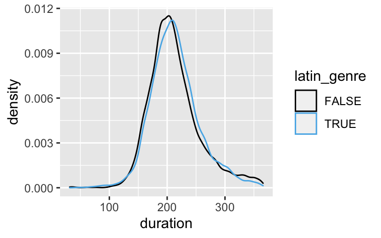
Researcher 2 – part 2
# Construct the model spotify_model_2 <- lm(duration ~ latin_genre, spotify_big) coef(summary(spotify_model_2)) ## Estimate Std. Error t value Pr(>|t|) ## (Intercept) 212.673908 0.4165491 510.56143 0.00000000 ## latin_genreTRUE 1.555355 0.7435700 2.09174 0.03647731On average, latin genre songs tend to be 1.56 seconds longer than edm / pop songs
No!
- Researcher 2 – part 3
- 0.03647731 / 2 = 0.018
- If there were truly no difference in the duration of latin vs pop / edm songs (in the broader population of songs), there’s only a p% chance that we’d have gotten a sample in which the observed difference was so large.
- We have statistically significant evidence that latin genre songs tend to be longer than pop / edm songs.
- Reflection
Large sample size! The more data we have, the smaller our standard errors. Thus the narrower our CIs and the smaller our p-values. Thus the easier it is to establish statistical significance even when the results aren’t practically significant.