8 Multivariate Modeling Principles
Announcements
- My Wednesday OH will be in the morning for the next 3 weeks. Please check the calendar on the online course manual.
- There are new preceptor OH on Thursday evenings. FB is a preceptor for Prof Grinde’s sections but can answer questions about our class and has access to my materials. Their OH are in person on the first floor reading room in the library.
- Checkpoint 8 is due Thursday. There are 2 videos. These recap and reiterate the concepts you’ll explore today. They don’t introduce new concepts.
- Homework 3 is due next Tuesday. I strongly encourage you to hand it in on Tuesday so that you can practice these concepts before the quiz.
- Quiz 1 is next Thursday. Please see details on page 7 of the syllabus. I recommend that you review each activity and homework, trying to answer the questions without first looking at your notes.
8.1 Getting started
WHERE ARE WE?
- You’ve seen most of the RStudio syntax we’ll need in this course. You’ll continue to apply and familiarize yourself with this code.
- We’re talking about multivariate relationships: modeling y by multiple predictors x. Why? If 2 or more predictors x both tell us about y, then maybe both together can tell us even more!
- Today:
- We’ll familiarize ourselves with the main ideas behind multivariate visualizations and modeling. You’ll explore these same ideas more deeply during our next classes.
- Remember to focus on the guiding principles (good for long-term retention, deeper understanding, and ability to generalize) as opposed memorizing “rules” (which don’t exist!).
- We’ll familiarize ourselves with the main ideas behind multivariate visualizations and modeling. You’ll explore these same ideas more deeply during our next classes.
EXAMPLE
Load some data:
# Load packages & import data
library(ggplot2)
library(dplyr)
bikes <- read.csv("https://www.macalester.edu/~dshuman1/data/155/bike_share.csv")
Take a quick peak at the results for four bivariate models of ridership, which will be referenced throughout the activity:
# Build and summarize some bivariate models
bike_model_1 <- lm(riders_registered ~ windspeed, bikes)
summary(bike_model_1)$r.squared
## [1] 0.04728406

bike_model_2 <- lm(riders_registered ~ temp_feel, bikes)
summary(bike_model_2)$r.squared
## [1] 0.2961447

bike_model_3 <- lm(riders_registered ~ weekend, bikes)
summary(bike_model_3)$r.squared
## [1] 0.07404211

bike_model_4 <- lm(riders_registered ~ season, bikes)
summary(bike_model_4)$r.squared
## [1] 0.2784603
Below, you will consider three more models, each of which has two predictors. The formulas for models 5, 6, & 7 will look like this:
bike_model_5:riders_registered= \(\beta_0\) + \(\beta_1\)windspeed+ \(\beta_2\)weekendTRUEbike_model_6:riders_registered= \(\beta_0\) + \(\beta_1\)weekendTRUE+ \(\beta_2\)seasonspring+ \(\beta_3\)seasonsummer+ \(\beta_4\)seasonwinterbike_model_7:riders_registered= \(\beta_0\) + \(\beta_1\)windspeed+ \(\beta_2\)temp_feel
Question: If we were to draw these formulas / models, what would they look like?
8.2 Exercises
DIRECTIONS
Since no rulebook exists, practice is extremely important to grasping multivariate models. After working through exercises 1-11, you’re strongly encouraged to: (1) work through the extra practice exercises at the end of the activity; and (2) review the solutions to all exercises in the online manual. Further, the two videos for our next class review some of these exercises.
- Hello!
What animal best represents how your week is going?
1 categorical & 1 quantitative predictor: visualization
Adjust the code below to recreate this visualization of the relationship ofriders_registeredwith the quantitativewindspeedpredictor and categoricalweekendpredictor.
ggplot(bikes, aes(y = riders_registered, x = windspeed)) +
  geom_point() +
  geom_smooth(method = "lm", se = FALSE)
1 categorical & 1 quantitative predictor: building a model
bike_model_5models the multivariate trend of riders vs windspeed and weekend:bike_model_5 <- lm(riders_registered ~ windspeed + weekend, bikes) summary(bike_model_5) ## ## Call: ## lm(formula = riders_registered ~ windspeed + weekend, data = bikes) ## ## Residuals: ## Min 1Q Median 3Q Max ## -3834.5 -951.3 -94.9 1158.5 3285.2 ## ## Coefficients: ## Estimate Std. Error t value Pr(>|t|) ## (Intercept) 4738.38 147.54 32.117 < 2e-16 *** ## windspeed -63.97 10.45 -6.120 1.53e-09 *** ## weekendTRUE -925.16 119.86 -7.718 3.89e-14 *** ## --- ## Signif. codes: 0 '***' 0.001 '**' 0.01 '*' 0.05 '.' 0.1 ' ' 1 ## ## Residual standard error: 1466 on 728 degrees of freedom ## Multiple R-squared: 0.1194, Adjusted R-squared: 0.1169 ## F-statistic: 49.33 on 2 and 728 DF, p-value: < 2.2e-16Thus the model formula is:
riders_registered = 4738.38053 - 63.97072 windspeed - 925.15701 weekendTRUE
What is the reference level of the
weekendpredictor?Confirm that
bike_model_5predicts roughly 3174 rides on weekend days when the windspeed is 10 mph and roughly 4099 rides on weekdays when the windspeed is 10 mph. Make sure you can match up these predictions with what you observe on the plot.# HINT # 4738.38053 - 63.97072*___ - 925.15701*___
1 categorical & 1 quantitative predictor: interpreting the model
We saw in exercise 2 that thebike_model_5formula (riders_registered = 4738.38053 - 63.97072 windspeed - 925.15701 weekendTRUE) is represented by two lines: one describing the relationship between rides and windspeed on weekends and the other on weekdays. This observation is key to interpretingbike_model_5!Utilize the model formula to identify the equations of these two lines. Hint: Plug
weekendTRUE = 0andweekendTRUE = 1.
weekdays: riders_registered = ___ - ___ windspeed
weekends: riders_registered = ___ - ___ windspeedReflecting on part a, let’s interpret what the model coefficients tell us about the physical properties of the two lines. Choose the correct option given in parentheses:
- The intercept coefficient, 4738.38, is the intercept of the line for (weekdays / weekends).
- The
windspeedcoefficent, -63.97, is the (intercept / slope) of both lines.
- The
weekendTRUEcoefficient, -925.16, indicates that the (intercept / slope) of the line for weekends is 925.16 riders lower than the (intercept / slope) of the line for weekdays. Similarly, since the lines are parallel, the line for weekends is 925.16 riders lower than the line weekdays at any windspeed.
Now that we’ve connected the 3 coefficients to the physical properties of the line, interpret each in a contextually meaningful way (i.e. what do they tell us about ridership?). Complete these sentences:
- Interpreting 4738.38: We expect roughly 4738 riders on ___ with 0 ___.
- Interpreting -63.97: On both weekends and weekdays…
- Interpreting -925.16: At any windspeed, we expect…
2 categorical predictors: visualization
Next, consider the relationship betweenriders_registeredand 2 categorical predictors:seasonandweekend. Adjust the code below to recreate this visualization of the relationship among these variables. HINT: color or fill

ggplot(bikes, aes(y = riders_registered, x = season)) +
  geom_boxplot()
2 categorical predictors: build & interpret the model
bike_model_6models the multivariate trend of riders vs season and weekend:bike_model_6 <- lm(riders_registered ~ weekend + season, bikes) summary(bike_model_6) ## ## Call: ## lm(formula = riders_registered ~ weekend + season, data = bikes) ## ## Residuals: ## Min 1Q Median 3Q Max ## -4240.4 -851.9 -194.1 1018.5 3051.9 ## ## Coefficients: ## Estimate Std. Error t value Pr(>|t|) ## (Intercept) 4260.45 99.16 42.964 < 2e-16 *** ## weekendTRUE -912.33 103.23 -8.838 < 2e-16 *** ## seasonspring -116.38 132.76 -0.877 0.380974 ## seasonsummer 438.44 132.06 3.320 0.000945 *** ## seasonwinter -1719.06 133.31 -12.896 < 2e-16 *** ## --- ## Signif. codes: 0 '***' 0.001 '**' 0.01 '*' 0.05 '.' 0.1 ' ' 1 ## ## Residual standard error: 1263 on 726 degrees of freedom ## Multiple R-squared: 0.3485, Adjusted R-squared: 0.345 ## F-statistic: 97.11 on 4 and 726 DF, p-value: < 2.2e-16Confirm that the model formula is:
riders_registered = 4260.45 - 912.33 weekendTRUE - 116.38 seasonspring + 438.44 seasonsummer - 1719.06 seasonwinterUse this model to predict the ridership on the following days:
# a fall weekday
# HINT: 4260.45 - 912.33*___ - 116.38*___  + 438.44*___ - 1719.06*___

# a winter weekday

# a fall weekend day

# a winter weekend day
How many possible predictions does this model produce?
Use these calculations and insights to fill in the below interpretations of the intercept coefficient,
weekendTRUEcoefficient, andseasonwintercoefficient. Hint: What is the meaning and consequence of plugging in 0 forweekendTRUE? Plugging in 1?- Interpreting 4260: We expect there to be 4260 riders on ___ during the ___.
- Interpreting -912: In any season, we expect there to be 912 ___ riders on weekends than on ___.
- Interpreting -1719: On both weekdays and weekends, we expect there to be 1719 ___ riders in winter than in ___.
2 quantitative predictors: visualization
Adjust the code below to recreate two visualizations of the relationship ofriders_registeredwith the quantitativewindspeedandtemp_feelpredictors.
ggplot(bikes, aes(y = riders_registered, x = windspeed)) +
  geom_point()
2 quantitative predictors: modeling
bike_model_7models the multivariate trend of riders vs windspeed and temperature:bike_model_7 <- lm(riders_registered ~ windspeed + temp_feel, bikes) summary(bike_model_7) ## ## Call: ## lm(formula = riders_registered ~ windspeed + temp_feel, data = bikes) ## ## Residuals: ## Min 1Q Median 3Q Max ## -3151.8 -975.8 -177.9 980.0 3273.8 ## ## Coefficients: ## Estimate Std. Error t value Pr(>|t|) ## (Intercept) -24.065 299.303 -0.080 0.935939 ## windspeed -36.544 9.408 -3.884 0.000112 *** ## temp_feel 55.516 3.331 16.668 < 2e-16 *** ## --- ## Signif. codes: 0 '***' 0.001 '**' 0.01 '*' 0.05 '.' 0.1 ' ' 1 ## ## Residual standard error: 1297 on 728 degrees of freedom ## Multiple R-squared: 0.3104, Adjusted R-squared: 0.3085 ## F-statistic: 163.9 on 2 and 728 DF, p-value: < 2.2e-16Thus the model formula is
riders_registered = -24.06 - 36.54windspeed + 55.52temp_feel
Confirm that this model predicts roughly 2941 rides on days when the windspeed is 10 mph and the temperature is 60 degrees. Try to match this up with the 3D plots in the next exercise.
- 2 quantitative predictors: interpreting the model
Thebike_model_7model formula is the formula of a plane (drawn below). CHALLENGE: Interpret the coefficients that define this plane (ie. the intercept,windspeed, andtemp_feelcoefficients frombike_model_7). HINTS:- In the left plot, the red arrows demonstrate the model trend at three different windspeeds (5, 20, and 30 mph). What are the slopes of these lines?
- In the right plot, the red arrows demonstrate the model trend at three different temperatures (40, 60, and 90 degrees). What are the slopes of these lines?

- In the left plot, the red arrows demonstrate the model trend at three different windspeeds (5, 20, and 30 mph). What are the slopes of these lines?
Which is best?
We’ve now seen 7 different models of ridership. Use the following table to answer the questions below.model predictors R2 bike_model_1windspeed0.047 bike_model_2temp_feel0.296 bike_model_3weekend0.074 bike_model_4season0.279 bike_model_5windspeed&weekend0.119 bike_model_6weekend&season0.349 bike_model_7windspeed&temp_feel0.310 - Which model does the best job of explaining the variability in ridership from day to day?
- If you could only pick one predictor, which would it be?
- What happens to R-squared when we add a second predictor to our model, and why does this make sense? For example, how does the R-squared for model 5 (with both windspeed and weekend) compare to those of model 1 (only windspeed) and model 3 (only weekend)?
- Are 2 predictors always better than 1? Provide evidence and explain why this makes sense.
- Reflection: principles of interpretation
These exercises have revealed some principles behind interpreting model coefficients. These are summarized below. Review and confirm that these make sense.
Principles of interpretation
A linear regression model describes the trend of a relationship between a response variable (\(y\)) and a set of predictors (\(x_1, x_2, ..., x_p\)). Suppose we have the following model without interaction terms (which we’ll learn about soon):
\[y = \beta_0 + \beta_1 x_1 + \beta_2 x_2 + \cdots + \beta_p x_p\]
Then we can interpret the coefficients as follows:
\(\beta_0\) (“beta 0”) is the y-intercept. It describes the typical value of \(y\) when \(x_1, x_2,..., x_k\) are all 0, ie. when all quantitative predictors are set to 0 and the categorical predictors are set to their reference levels.
\(\beta_i\) (“beta i”) is the coefficient of \(x_i\).
- If \(x_i\) is quantitative, \(\beta_i\) describes the typical change in \(y\) per 1-unit increase in \(x_i\) while at a fixed set of the other \(x\).
- If \(x_i\) represents a category of a categorical variable, \(\beta_i\) describes the typical change in \(y\) when we move to this category from the reference category while at a fixed set of the other \(x\).
- If \(x_i\) is quantitative, \(\beta_i\) describes the typical change in \(y\) per 1-unit increase in \(x_i\) while at a fixed set of the other \(x\).
8.2.1 Extra practice
NOTE: The video for tomorrow will go through practice exercises 1 through 4.
- Curiosity!
In working through the exercises, you probably had an “I wonder…” moment or two. What were they? What else do you want to learn about these data? Try it!
- Practice 1
Consider the relationship ofriders_registeredvsweekendandweather_cat.- Construct a visualization of this relationship.
- Construct a model of this relationship.
- Interpret the first 3 model coefficients.
- Construct a visualization of this relationship.
- Practice 2
Consider the relationship ofriders_registeredvstemp_feelandhumidity.- Construct a visualization of this relationship.
- Construct a model of this relationship.
- Interpret the first 3 model coefficients.
- Construct a visualization of this relationship.
- Practice 3
Consider the relationship ofriders_registeredvstemp_feelandweather_cat.- Construct a visualization of this relationship.
- Construct a model of this relationship.
- Interpret the first 3 model coefficients.
- Construct a visualization of this relationship.
- Practice 4: CHALLENGE
We’ve looked at models with 2 predictors. What about 3 predictors?! Consider the relationship ofriders_registeredvstemp_feel,humidity, ANDweekend.- Construct a visualization of this relationship.
- Construct a model of this relationship.
- Interpret each model coefficient.
- If you had to draw the shape of the model trend, what would it look like: a line, parallel lines, a plane, parallel planes?
- Construct a visualization of this relationship.
8.3 Solutions
- Hello!
1 categorical & 1 quantitative predictor: visualization
ggplot(bikes, aes(y = riders_registered, x = windspeed, color = weekend)) +
  geom_point() +
  geom_smooth(method = "lm", se = FALSE)
- 1 categorical & 1 quantitative predictor: building a model
riders_registered = 4738.38 - 63.97 windspeed - 925.16 weekendTRUE
weekend FALSE (i.e. weekdays)
.
4738.38 - 63.97*10 - 925.16*1
## [1] 3173.52
4738.38 - 63.97*10 - 925.16*0
## [1] 4098.68
- 1 categorical & 1 quantitative predictor: interpreting the model
weekdays: riders_registered = 4738.38 - 63.97 windspeed
weekends: riders_registered = 4738.38 - 63.97 windspeed - 925.16 = 3813.22 - 63.97 windspeed.
- The intercept coefficient, 4738.38, is the intercept of the line for weekdays.
- The
windspeedcoefficent, -63.97, is the slope of both lines. - The
weekendTRUEcoefficient, -925.16, indicates that the intercept of the line for weekends is 925.16 riders lower than the intercept of the line for weekdays. Similarly, since the lines are parallel, the line for weekends is 925.16 riders lower than the line weekdays at any windspeed.
.
- We expect roughly 4738 riders on weekdays with 0 windspeed.
- On both weekends and weekdays, we expect 64 fewer riders for every 1mph increase in windspeed.
- At any windspeed, we expect 925 fewer riders on weekend days than on weekdays.
2 categorical predictors: visualization
ggplot(bikes, aes(y = riders_registered, x = season, fill = weekend)) +
  geom_boxplot()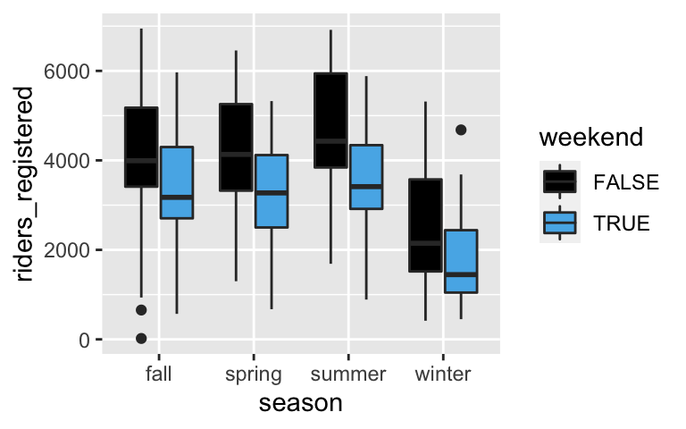
- 2 categorical predictors: build & interpret the model
.
#fall weekday:
4260.45 - 912.33*0 - 116.38*0 + 438.44*0 - 1719.06*0
## [1] 4260.45

#winter weekday:
4260.45 - 912.33*0 - 116.38*0 + 438.44*0 - 1719.06*1
## [1] 2541.39

#fall weekend:
4260.45 - 912.33*1 - 116.38*0 + 438.44*0 - 1719.06*0
## [1] 3348.12

#winter weekend:
4260.45 - 912.33*1 - 116.38*0 + 438.44*0 - 1719.06*1
## [1] 1629.06
8: 2 weekend categories * 4 season categories
.
- We expect there to be 4260 riders on weekdays during the fall.
- In any season, we expect there to be 912 fewer riders on weekends than on weekdays.
- On both weekdays and weekends, we expect there to be 1719 fewer riders in winter than in fall.
2 quantitative predictors: visualization
ggplot(bikes, aes(y = riders_registered, x = windspeed, size = temp_feel)) +
  geom_point()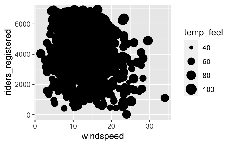
ggplot(bikes, aes(y = riders_registered, x = windspeed, color = temp_feel)) +
  geom_point()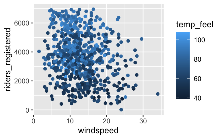
- 2 quantitative predictors: modeling
riders_registered = -24.065 - 36.544windspeed + 55.516temp_feel
.
-24.065 - 36.544*10 + 55.516*60
## [1] 2941.455
- 2 quantitative predictors: interpreting the model
- -24.065 = typical ridership on days with 0 windspeed and a 0 degree temperature. (This doesn’t make contextual sense, but indicates where the plane “lives” in space!)
- -36.544 = no matter the temperature, we expect 37 fewer riders for every 1mph increase in windspeed
- 55.516 = no matter the windspeed, we expect 56 more riders for every 1 degree increase in temperature
- Which is best?
- model 6
- temperature
- R-squared increases (our model is stronger when we include another predictor)
- nope. model 5 (with windspeed and weekend) has a lower R-squared than model 2 (with only temperature)
- …
- …
Practice 1
ggplot(bikes, aes(y = riders_registered, x = weekend, fill = weather_cat)) +
  geom_boxplot()
new_model_1 <- lm(riders_registered ~ weekend + weather_cat, bikes) coef(summary(new_model_1)) ## Estimate Std. Error t value Pr(>|t|) ## (Intercept) 4211.8741 75.54724 55.751529 9.461947e-265 ## weekendTRUE -982.2106 117.24719 -8.377264 2.786301e-16 ## weather_catcateg2 -608.8640 113.00211 -5.388077 9.628947e-08 ## weather_catcateg3 -2360.2049 319.71640 -7.382183 4.270163e-13- The typical ridership on a weekday with nice weather (categ1) is 4212 rides.
- On days with similar weather, the typical ridership on a weekend is 982 rides less than on weekdays.
- On similar days of the week, the typical ridership when the weather is “dreary” (categ2) is 609 rides less than when the weather is nice.
- The typical ridership on a weekday with nice weather (categ1) is 4212 rides.
Practice 2
ggplot(bikes, aes(y = riders_registered, x = temp_feel, color = humidity)) +
    geom_point()
new_model_2 <- lm(riders_registered ~ temp_feel + humidity, bikes) coef(summary(new_model_2)) ## Estimate Std. Error t value Pr(>|t|) ## (Intercept) 315.83704 303.777334 1.039699 2.988249e-01 ## temp_feel 60.43316 3.272315 18.468015 9.451345e-63 ## humidity -1868.99356 336.963661 -5.546573 4.078901e-08- It doesn’t really make sense to interpret the intercept – we didn’t see any days that were 0 degrees with 0 humidity.
- On days with similar humidity, the typical ridership increases by 60 rides for each 1 degree increase in temperature.
- On days with similar temperature, the typical ridership decreases by 1867 * 0.1 = 187 rides for each 0.1 increase in humidity levels.
- It doesn’t really make sense to interpret the intercept – we didn’t see any days that were 0 degrees with 0 humidity.
Practice 3
new_model_3 <- lm(riders_registered ~ temp_feel + weather_cat, bikes)
coef(summary(new_model_3))
##                      Estimate Std. Error   t value     Pr(>|t|)
## (Intercept)        -288.68840 251.264383 -1.148943 2.509574e-01
## temp_feel            55.30133   3.215495 17.198387 7.082670e-56
## weather_catcateg2  -386.42241 100.187725 -3.856984 1.249775e-04
## weather_catcateg3 -1919.01375 283.022420 -6.780430 2.481218e-11

ggplot(bikes, aes(y = riders_registered, x = temp_feel, color = weather_cat)) +
    geom_point() +
    geom_line(aes(y = new_model_3$fitted.values), size = 1.5)
- It doesn’t really make sense to interpret the intercept – we didn’t see any days that were 0 degrees.
- On days with similar weather, the typical ridership increases by 55 rides for each 1 degree increase in temperature.
- On days with similar temperature, the typical ridership is 386 rides lower on a dreary weather day (categ2) than a nice weather day (categ1).
- It doesn’t really make sense to interpret the intercept – we didn’t see any days that were 0 degrees.
Practice 4
new_model_4 <- lm(riders_registered ~ temp_feel + humidity + weekend, bikes)
coef(summary(new_model_4))
##                Estimate Std. Error   t value     Pr(>|t|)
## (Intercept)   668.60236 292.181063  2.288315 2.240530e-02
## temp_feel      59.36751   3.119256 19.032585 7.626695e-66
## humidity    -1906.43437 320.982938 -5.939364 4.433789e-09
## weekendTRUE  -869.05771 100.057822 -8.685555 2.471050e-17

ggplot(bikes, aes(y = riders_registered, x = temp_feel, color = weekend, size = humidity)) +
  geom_point()
- It doesn’t really make sense to interpret the intercept – we didn’t see any days that were 0 degrees.
- On days with similar humidity and time of week, the typical ridership increases by 59 rides for each 1 degree increase in temperature.
- On days with similar temperature and time of week, the typical ridership decreases by 1906*0.1 = 190.6 rides for each 0.1 point increase in humidity levels.
- On days with similar temperature and humidity, the typical ridership is 869 rides lower on weekends vs weekdays.
This model would look like 2 parallel planes, one for weekends and one for weekdays! Why?
riders_registeredvstemp_feel(quant) would be a line. Adding inhumidity(quant) would turn the model into a plane. Adding inweekend(cat) would split this one plane into two unique planes, one for each weekend category!- It doesn’t really make sense to interpret the intercept – we didn’t see any days that were 0 degrees.