11 Simpson’s Paradox (optional)
Goals
In this unit we’ve been exploring multivariate statistical models. Upon learning how to interpret these models, we’ve examined their potential benefits and potential pitfalls (eg: multicollinearity, overfitting). In today’s activity, you’ll learn about another fun kind of puzzle we can run into in multivariate analyses: a Simpson’s Paradox occurs when the sign (+/-) of a coefficient, thus the meaning of the relationship, changes when controlling for a new covariate. This switch can typically be explained by a confounding variable, ie. a variable that affects the relationship among the variables of primary interest. Not controlling for a confounding variable may result in a misleading interpretation of the relationship of interest.
Note
This material is fun but optional. You’re encouraged to take ownership of your learning. If your time would be better spent on reviewing former material and working on homework, please do so. If you are looking for a new challenge / to learn a new concept, please continue with the exercises below. The only thing that’s not an option is to not use this time to dig into STAT 155 material.
11.1 Exercises
In the exercises below, you’ll explore data on diamonds – these data provide a good illustration of Simpson’s Paradox. The diam data set contains data on price, carat (size), color, and clarity (quality) of 308 diamonds:
diam <- read.csv("https://www.macalester.edu/~ajohns24/data/Diamonds.csv")We want to explore the extent to which a diamond’s price depends upon its clarity (a measure of quality). Clarity is classified as follows, in order from best to worst:
| Clarity | Description |
|---|---|
| IF | flawless (no internal imperfections) |
| VVS1 | very very slightly imperfect |
| VVS2 | " " |
| VS1 | very slightly imperfect |
| VS2 | " " |
- Gut check
Before looking at the data, what do your instincts say?- Do flawless (higher clarity) diamonds tend to cost more or less than flawed (lower clarity) diamonds?
- Do bigger diamonds cost more or less than smaller diamonds?
- Do bigger diamonds tend to have more or fewer flaws (lower or higher clarity)?
- Do flawless (higher clarity) diamonds tend to cost more or less than flawed (lower clarity) diamonds?
pricevsclarity
Let’s see what the data say. Which clarity level tends to cost the most? Which clarity level tends to cost the least? Support your answers with:- graphical evidence
- numerical evidence from a model of
price ~ clarity
- graphical evidence
pricevsclarityandcarat
These surprising results can be explained by a confounding variable:carat(ie. the size of a diamond). To see why:- construct a model of
price ~ clarity + carat
- construct a plot of
pricevsclarityandcarat. Include a representation of your model usinggeom_line(aes(y = YOURMODEL$fitted.values), size = 1.5)
- construct a model of
Making sense of this model
Inspect the model coefficients. What do you think now?- Which clarity costs the most? (Give some numerical evidence from the model.)
- Which clarity costs the least? (Give some numerical evidence from the model.)
- Which clarity costs the most? (Give some numerical evidence from the model.)
Simpson’s Paradox
Theclaritycoefficients in the model of price when we don’t control forcarathave the opposite sign as the coefficients when we do control forcarat. This is called a Simpson’s paradox. Explain why this happened. Support your argument with new graphical evidence.
HINT
Perfect IF diamonds seemed cheaper, but only because IF diamonds tend to be ??? and ??? diamonds are cheaper.
- Final conclusion
Based on these observations alone, what’s your conclusion about diamond prices?- flawed diamonds are more expensive
- flawless diamonds are more expensive
11.2 Solutions
- Gut check
Your gut might differ, but here’s what mine says:- Do flawless (higher clarity) diamonds tend to cost more or less than flawed (lower clarity) diamonds? More.
- Do bigger diamonds cost more or less than smaller diamonds? More.
- Do bigger diamonds tend to have more or fewer flaws (lower or higher clarity)? More – there’s more volume and so more opportunities for flaws.
- Do flawless (higher clarity) diamonds tend to cost more or less than flawed (lower clarity) diamonds? More.
pricevsclarity
Most: VS2 (it costs $3163.40 more than an IF diamond on average)
Least: IF (it costs only $2694.773 on average)ggplot(diam, aes(y = price, x = clarity)) + geom_boxplot()
model_1 <- lm(price ~ clarity, diam)
coef(summary(model_1))
##             Estimate Std. Error  t value     Pr(>|t|)
## (Intercept) 2694.773   494.1723 5.453103 1.028429e-07
## clarityVS1  2362.264   613.8905 3.848022 1.452275e-04
## clarityVS2  3163.397   668.5384 4.731810 3.418595e-06
## clarityVVS1 2872.862   671.4480 4.278607 2.524997e-05
## clarityVVS2 2661.779   618.0321 4.306861 2.239541e-05
pricevsclarityandcaratmodel_2 <- lm(price ~ clarity + carat, diam) coef(summary(model_2)) ## Estimate Std. Error t value Pr(>|t|) ## (Intercept) -1851.2127 177.5113 -10.428703 5.968191e-22 ## clarityVS1 -1001.1529 202.9952 -4.931906 1.346709e-06 ## clarityVS2 -1561.8944 228.2176 -6.843884 4.300638e-11 ## clarityVVS1 -403.6762 219.7444 -1.837026 6.718861e-02 ## clarityVVS2 -958.8220 205.8089 -4.658797 4.775083e-06 ## carat 12226.3668 232.1566 52.664305 3.083330e-154 ggplot(diam, aes(y = price, x = carat, color = clarity)) + geom_point() + geom_line(aes(y = model_2$fitted.values), size = 1.5)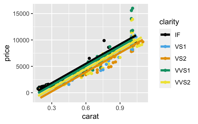
- Making sense of this model
- IF costs the most. When controlling for the size of a diamond (carat), all other clarities cost less than IF on average (they have negative coefficients).
- VS2 costs the least. When controlling for the size of a diamond (carat), VS2 diamonds cost $1561.89 less than IF diamonds on average.
Simpson’s Paradox
Perfect IF diamonds seemed cheaper, but only because IF diamonds tend to be smaller and smaller diamonds are cheaper.# IF tend to be smaller ggplot(diam, aes(y = carat, x = clarity)) + geom_boxplot()
# Smaller diamonds tend to be cheaper
ggplot(diam, aes(y = price, x = carat)) +
    geom_point()
- Final conclusion
flawless diamonds are more expensive