13 Logistic regression: Part I
Announcements
Homework 4 is due today. The extension closes on Sunday at 9:30am.
Checkpoint 11 is due Thursday.
Nothing is due the Tuesday after spring break.
Checkpoint 12 and Homework 5 are due the Thursday after spring break.
Mac is holding our sixth DataFest on March 25-27, 2022. DataFest is a nationally-coordinated undergraduate competition in which teams of two to five students work over a weekend to extract insight from a rich and complex data set. Previous years’ data sets have included crime data from the LAPD, dating data from eHarmony, energy use data from GridPoint, and travel data from Expedia. This year’s data will be revealed at the opening of the event.
We encourage students to form teams with a diverse set of skills and backgrounds (e.g., a blend of experiences in data computing, statistics, GIS, visualization and the arts, and business and economics). Those with no data science experience are welcome. Looking to join a team or add teammates? Indicate that on the registration form.
13.1 Getting started
Where are we?
We’ve been focusing on “Normal” linear regression models for quantitative response variables. But not all response variables are quantitative! We’ll now explore logistic regression models for binary categorical response variables. Though the details of our models will change, the spirit and considerations are the same:
- we want to learn about y from predictors x
- we want to build, interpret, and evaluate our models
- we need to be mindful of multicollinearity, overfitting, etc in this process
Logistic Regression
Let \(y\) be a binary categorical response variable:
\[y = \begin{cases} 1 & \; \text{ if event happens} \\ 0 & \; \text{ if event doesn't happen} \\ \end{cases}\]
Further define
\[\begin{split} p &= \text{ probability event happens} \\ 1-p &= \text{ probability event doesn't happen} \\ \text{odds} & = \text{ odds event happens} = \frac{p}{1-p} \\ \end{split}\]
Then a logistic regression model of \(y\) by \(x\) is \[\log(\text{odds}) = \beta_0 + \beta_1 x\]
We can transform this to get (curved) models of odds and probability:
\[\begin{split} \text{odds} & = e^{\beta_0 + \beta_1 x} \\ p & = \frac{\text{odds}}{\text{odds}+1} = \frac{e^{\beta_0 + \beta_1 x}}{e^{\beta_0 + \beta_1 x}+1} \\ \end{split}\]
Warm-up 1: Normal or logistic?
For each scenario below, indicate whether Normal or logistic regression would be the appropriate modeling tool.
- scenario 1: we want to model a person’s commute time (y) by their distance to work (x).
- scenario 2: we want to model a person’s commute time (y) by whether or not they take public transit (x).
- scenario 3: we want to model whether or not a person gets a speeding ticket (y) based on their driving speed (x).
Warm-up 2: probability vs odds vs log(odds)
- Let p denote the probability of an event. Identify examples of events for which: p = 0 and p = 1.
- There’s a 0.9 probability that your team wins the next game. Calculate the corresponding odds and log(odds) of this event. NOTE:
log()is the natural log function in RStudio.
- The log(odds) that your bus is late are -1. Calculate the corresponding odds and probability of this event. NOTE: Use
exp().
13.2 Exercises
Directions
There’s a lot of new and specialized syntax today. Not even I have this syntax committed to memory. During class, you’re encouraged to peak at but not get distracted by the syntax – stay focused on the bigger picture concepts. After the activity, go back and pick through the syntax.
Reminders
- Make mistakes!
- Support one another and stay in sync! You should be discussing each exercise as you go.
- If you don’t finish the activity during class, be sure to revisit after class and check the online solutions.
The story
The climbers_sub data is sub-sample of the Himalayan Database distributed through the R for Data Science TidyTuesday project. This dataset includes information on the results and conditions for various Himalayan climbing expeditions. Each row corresponds to a single member of a climbing expedition team:
# Load packages and data
library(ggplot2)
library(dplyr)
climbers_sub <- read.csv("https://www.macalester.edu/~ajohns24/data/climbers_sub.csv") %>%
  select(peak_name, success, age, oxygen_used, height_metres)

# Check out the first 6 rows
head(climbers_sub)
##    peak_name success age oxygen_used height_metres
## 1 Ama Dablam    TRUE  28       FALSE          6814
## 2 Ama Dablam    TRUE  27       FALSE          6814
## 3 Ama Dablam    TRUE  35       FALSE          6814
## 4 Ama Dablam    TRUE  37       FALSE          6814
## 5 Ama Dablam    TRUE  43       FALSE          6814
## 6 Ama Dablam   FALSE  38       FALSE          6814
Our goal will be to model whether or not a climber has success by their age. Since success is a binary categorical variable (a climber is either successful or they’re not), we’ll utilize logistic regression.
- Hello!
What’s your spring break plan?
A quick peak at the data
# How many climbers are in the data set?

# Overall, how many climbers succeeded / didn't succeed? Hint: count()
Plotting success by age
It’s not often easy to visualize a relationship between a binary response y and a predictor x. But since we have a large data set and multiple (though sometimes not many) observations at each age, we can calculate the observed success rate at each age. Try out the plots below and summarize what you learn.# Calculate success rate by age # And plot success rate by age success_by_age <- climbers_sub %>% group_by(age) %>% summarize(success_rate = mean(success)) ggplot(success_by_age, aes(x = age, y = success_rate)) + geom_point() # Do the above in 1 set of lines! climbers_sub %>% group_by(age) %>% summarize(success_rate = mean(success)) %>% ggplot(aes(x = age, y = success_rate)) + geom_point() # Split climbers into larger, more stable age brackets # (This is good when we don't have many / multiple observations at each x!) # Plot success rate by age bracket climbers_sub %>% mutate(age_bracket = cut(age, breaks = 20)) %>% group_by(age_bracket) %>% summarize(success_rate = mean(success)) %>% ggplot(aes(x = age_bracket, y = success_rate)) + geom_point()
Logistic regression in R
To model the relationship betweensuccessandage, we can construct the logistic regression model. NOTE: For logistic regression we useglm()instead oflm()and usefamily = "binomial"to specify that our response variable is binary.climbing_model_1 <- glm(success ~ age, data = climbers_sub, family = "binomial") coef(summary(climbing_model_1))Convince yourself that the model formulas on the log(odds), odds, and probability scales are as follows:
log(odds of success) = 0.42569 - 0.02397age
odds of success = e^(0.42569 - 0.02397age)
probability of success = e^(0.42569 - 0.02397age) / (e^(0.42569 - 0.02397age) + 1)
Plotting the model
We now have the same model of success by age, but on 3 different scales. Construct and comment on the plots below – what do they indicate about the relationship between climber success and age?# Incorporate predictions on the probability, odds, & log-odds scales climbers_predictions <- climbers_sub %>% mutate(probability = climbing_model_1$fitted.values) %>% mutate(odds = probability / (1-probability)) %>% mutate(log_odds = log(odds)) # Plot the model on the log-odds scale ggplot(climbers_predictions, aes(x = age, y = log_odds)) + geom_smooth(se = FALSE) # Plot the model on the odds scale ggplot(climbers_predictions, aes(x = age, y = odds)) + geom_smooth(se = FALSE) # Plot the model on the probability scale ggplot(climbers_predictions, aes(x = age, y = probability)) + geom_smooth(se = FALSE) #...and zoom out to see broader (and impossible) age range ggplot(climbers_predictions, aes(x = age, y = as.numeric(success))) + geom_smooth(method = "glm", method.args = list(family = "binomial"), se = FALSE, fullrange = TRUE) + labs(y = "probability") + lims(x = c(-200,200))
- Interpreting the plots
Compare the shapes of the models on these different scales.
a. Which model is linear?
b. Which model is s-shaped?
c. Which model is restricted between 0 and 1 on the y-axis?
d. Which model is curved and restricted to be above 0 (but not necessarily below 1) on the y-axis?
Predictions
Recall our model on 3 scales:log(odds of success) = 0.42569 - 0.02397age
odds of success = e^(0.42569 - 0.02397age)
probability of success = e^(0.42569 - 0.02397age) / (e^(0.42569 - 0.02397age) + 1)Let’s use the model to make predictions. Consider a 20-year-old climber.
- Predict the log(odds) that this climber will succeed. HINT: use the log(odds) model.
- Predict the odds that this climber will succeed. HINT: Either transform the log(odds) prediction or use the odds model.
- Predict the probability that this climber will succeed. HINT: Either transform the odds prediction or use the probability model.
- Predict the log(odds) that this climber will succeed. HINT: use the log(odds) model.
- Checking predictions
On each of the 3 scales, are your predictions consistent with your model visualizations above?
Check your predictions using the following picky syntax.
# Check the log-odds prediction
predict(climbing_model_1, newdata = data.frame(age = 20))

# Check the odds prediction
exp(predict(climbing_model_1, newdata = data.frame(age = 20)))

# Check the probability prediction
predict(climbing_model_1, newdata = data.frame(age = 20), type = "response")
- Interpreting Coefficients
You’ll learn more in the next checkpoint about interpreting logistic regression coefficients. Give it a quick try here.- Interpret the intercept coefficient on the log(odds) scale. NOTE: You can do this just as you did for “Normal” regression models, but remember that the response here is log(odds of success).
- Interpret the intercept coefficient on the odds scale. HINT:
exp()
- Interpret the
agecoefficient on the log(odds) scale. NOTE: You can do this just as you did for “Normal” regression models, but remember that the response here is log(odds of success).
- CHALLENGE: The log(odds) scale isn’t very nice. We can convert this to the odds scale as follows. If the
agecoefficient on the log(odds) scale is b, then e^b is the MULTIPLICATIVE change in ODDS of success per 1 year increase in age. For example, if e^b = 2, then the odds of success double with each additional year in age. With this, interpret theagecoefficient on the odds scale.
- OPTIONAL MATH CHALLENGE: Try to prove the relationship used in part d.
- Interpret the intercept coefficient on the log(odds) scale. NOTE: You can do this just as you did for “Normal” regression models, but remember that the response here is log(odds of success).
- Another climbing model
a. Construct a logistic regression model ofsuccessbyoxygen_used.
b. Predict the probability of success for a climber that uses oxygen and for a climber that doesn’t use oxygen.
c. CHALLENGE: Interpret the two model coefficients.
13.3 Solutions
Warm-up: probability vs odds vs log(odds)
# a. will vary

# b
# odds
0.9 / (1 - 0.9)
## [1] 9
# log(odds)
log(0.9 / (1 - 0.9))
## [1] 2.197225

# c
# odds
exp(-1)
## [1] 0.3678794
# prob
exp(-1) / (exp(-1) + 1)
## [1] 0.2689414
A quick peak at the data
# How many climbers are in the data set?
nrow(climbers_sub)
## [1] 2076

# Overall, how many climbers succeeded / didn't succeed? Hint: n()
climbers_sub %>%
  count(success)
##   success    n
## 1   FALSE 1269
## 2    TRUE  807
Plotting success by age
Success rate is lower among older climbers# Calculate success rate by age # And plot success rate by age success_by_age <- climbers_sub %>% group_by(age) %>% summarize(success_rate = mean(success)) ggplot(success_by_age, aes(x = age, y = success_rate)) + geom_point()
# Do the above in 1 set of lines!
climbers_sub %>%
  group_by(age) %>%
  summarize(success_rate = mean(success)) %>%
  ggplot(aes(x = age, y = success_rate)) +
    geom_point()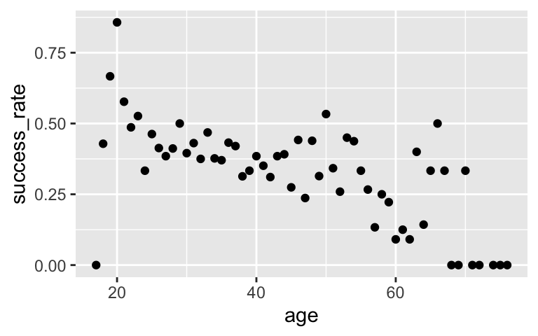
# Split climbers into larger, more stable age brackets
# (This is good when we don't have many / multiple observations at each x!)
# Plot success rate by age bracket
climbers_sub %>%
  mutate(age_bracket = cut(age, breaks = 20)) %>%
  group_by(age_bracket) %>%
  summarize(success_rate = mean(success)) %>%
  ggplot(aes(x = age_bracket, y = success_rate)) +
    geom_point() +
    theme(axis.text.x = element_text(angle = 90, vjust = 0.5, hjust=1))
Logistic regression in R
These are the definitions.climbing_model_1 <- glm(success ~ age, data = climbers_sub, family = "binomial") coef(summary(climbing_model_1)) ## Estimate Std. Error z value Pr(>|z|) ## (Intercept) 0.42568563 0.169177382 2.516209 1.186249e-02 ## age -0.02397199 0.004489504 -5.339564 9.317048e-08
Plotting the model
Success rate is lower among older climbers# Incorporate predictions on the probability, odds, & log-odds scales climbers_predictions <- climbers_sub %>% mutate(probability = climbing_model_1$fitted.values) %>% mutate(odds = probability / (1-probability)) %>% mutate(log_odds = log(odds)) # Plot the model on 3 scales ggplot(climbers_predictions, aes(x = age, y = log_odds)) + geom_smooth(se = FALSE) ggplot(climbers_predictions, aes(x = age, y = odds)) + geom_smooth(se = FALSE) ggplot(climbers_predictions, aes(x = age, y = probability)) + geom_smooth(se = FALSE) #...and zoom out to see broader (and impossible) age range ggplot(climbers_predictions, aes(x = age, y = as.numeric(success))) + geom_smooth(method = "glm", method.args = list(family = "binomial"), se = FALSE, fullrange = TRUE) + labs(y = "probability") + lims(x = c(-200,200))
- Interpreting the plots
a. log(odds) model
b. probability model
c. probability model
d. odds model
Predictions
#a
0.42568563 - 0.02397199 * 20
## [1] -0.05375417

#b
exp(0.42568563 - 0.02397199 * 20)
## [1] 0.947665

#c
exp(0.42568563 - 0.02397199 * 20) / (exp(0.42568563 - 0.02397199 * 20) + 1)
## [1] 0.4865647
Checking predictions
# Check the log-odds prediction
predict(climbing_model_1, newdata = data.frame(age = 20))
##           1
## -0.05375421

# Check the odds prediction
exp(predict(climbing_model_1, newdata = data.frame(age = 20)))
##        1
## 0.947665

# Check the probability prediction
predict(climbing_model_1, newdata = data.frame(age = 20), type = "response")
##         1
## 0.4865647
- Interpreting Coefficients
- At age 0 (doesn’t make sense), the typical log(odds of success) is 0.426
- At age 0 (doesn’t make sense), the typical odds of success are 1.63 (e0.426)
- For every 1 year increase in age, log(odds of success) decrease by 0.024.
- For every 1 year increase in age, odds of success are 97.6% as high (e(-0.024)) decrease by 0.024.
- Another climbing model
In c, the odds of success when not using oxygen are 0.26. The odds of success when using oxygen are 18 times higher.
```r
#a
climbing_model_2 <- glm(success ~ oxygen_used, data = climbers_sub, family = "binomial")
coef(summary(climbing_model_2))
##                  Estimate Std. Error   z value      Pr(>|z|)
## (Intercept)     -1.327993  0.0639834 -20.75528  1.098514e-95
## oxygen_usedTRUE  2.903864  0.1257404  23.09412 5.304291e-118

#b
#no oxygen
exp(-1.33) / (exp(-1.33) + 1)
## [1] 0.2091594
#oxygen
exp(-1.33 + 2.90) / (exp(-1.33 + 2.90) + 1)
## [1] 0.8277836

#c
exp(-1.33)
## [1] 0.2644773
exp(2.90)
## [1] 18.17415
```
- Another climbing model
.
climbing_model_1 <- glm(success ~ oxygen_used, data = climbers_sub, family = "binomial")
coef(summary(climbing_model_1))
##                  Estimate Std. Error   z value      Pr(>|z|)
## (Intercept)     -1.327993  0.0639834 -20.75528  1.098514e-95
## oxygen_usedTRUE  2.903864  0.1257404  23.09412 5.304291e-118
83% vs 21% chance of success. A big difference!
# Uses oxygen
exp(-1.327993 + 2.903864) / (1 + exp(-1.327993 + 2.903864))
## [1] 0.828619

# Doesn't use oxygen
exp(-1.327993) / (1 + exp(-1.327993))
## [1] 0.2094915
Will discuss this type of question on Thursday.