20 Hypothesis testing

Announcements

Upcoming due dates:

Today: Mini-project Phase 1. The last time that you can hand this in for credit is on Thursday (2 days from now). There’s less flexibility here than with homework, since you’ll need to move on to Phase 2!
Thursday: Checkpoint 17
Next Thursday, April 21: Homework 7 (last homework!) & Mini-project Phase 2
Tuesday, April 26 (2 weeks from today): Quiz 3. This will be the same as Quizzes 1 & 2 except the second part will be due by 10pm on the same day, not the next day.

Other things:

I want to hear from more people again! I will assign each table an example to discuss with the class.
Fall 2022 registration is around the corner. Please reach out with any questions you have about MSCS classes (or anything else really!). Here are some highlights:
- COMP / STAT 112: Intro to Data Science
  This is similar in vibe to STAT 155, but digs deeper into data wrangling (dplyr-ish stuff) and visualization (ggplot stuff).
- STAT 125: Epidemiology
  This course is at the intersection of public health and statistics. Though it discusses statistical concepts, it is less technical than STAT 155 (eg: less RStudio).
- STAT 253: Statistical Machine Learning
  Building upon STAT 155, this course surveys a range of other modeling tools, algorithms, and techniques. As a sequel to 155, it moves a bit faster and goes a bit deeper.

20.1 Getting started

The whole point

we can use sample data to estimate features of the population
there’s error in this estimation
taking this error into account, what exactly can we conclude about the population?

Data story

Consider data on wages:

# Load packages
library(ggplot2)
library(dplyr)
library(mosaic)

# Load the data
CPS_2018 <- read.csv("https://www.macalester.edu/~ajohns24/data/CPS_2018.csv")

We’ll start our wage analysis by exploring the population model of wages by age:

\[\text{wage} = \beta_0 + \beta_1 \text{ age}\]

where $\beta_0$ and $\beta_1$ are unknown population coefficients. (After all, we don’t know the wage & age of everybody in the labor force!) Let’s estimate the wage model using our sample data:

# Model the relationship
wage_model_1 <- lm(wage ~ age, data = CPS_2018)
coef(summary(wage_model_1))
##               Estimate Std. Error  t value     Pr(>|t|)
## (Intercept) 27954.3732 2146.56299 13.02285 1.862909e-38
## age           548.7934   47.89052 11.45933 3.258478e-30

# Plot the model
ggplot(CPS_2018, aes(x = age, y = wage)) + 
  geom_smooth(method = "lm")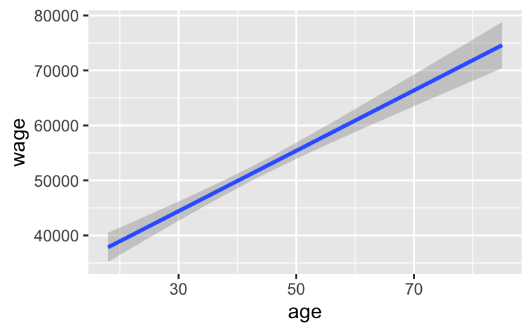

NOTES:

We estimate that wage increases by $548.79 on average for every 1 year increase in age.
This estimate has a standard error of 47.89. That is, among samples like ours, the typical error among age coefficient estimates is likely around 47.89 (dollars per year). Or more simply, we expect that our estimate might be off by 47.89.

EXAMPLE 1

Consider the 95% confidence intervals for the (unknown) population coefficients:

confint(wage_model_1)
##                  2.5 %     97.5 %
## (Intercept) 23746.6777 32162.0688
## age           454.9184   642.6685

How can we interpret the CI for the age coefficient?
- There’s a 95% chance that, in the broader labor force, wage increases somewhere between $454.92 and $642.67 for every 1 year increase in age, on average.
- We’re 95% confident that, in the broader labor force, wage increases somewhere between $454.92 and $642.67 for every 1 year increase in age, on average.
- We’re 95% confident that, in our sample, wage increases somewhere between $454.92 and $642.67 for every 1 year increase in age, on average.
Does this CI provide statistically significant evidence that, on average, wage increases with age?

EXAMPLE 2: Step 1 – specify the hypotheses

Let’s move on to a more formal hypothesis test. A researcher states the following hypotheses about the (unknown) population age coefficient $\beta_1$:

H_0: $\beta_1 = 0$
H_a: $\beta_1 > 0$

How can we interpret these hypotheses?

H_0: On average, wage increases with age.
H_a: There’s no association between wage and age.

H_0: On average, wage decreases with age.
H_a: There’s no association between wage and age.

H_0: There’s no association between wage and age.
H_a: On average, wage increases with age.

H_0: There’s no association between wage and age.
H_a: On average, wage decreases with age.

PAUSE for a thought experiment

Innocent until proven guilty. In Step 2 of the hypothesis test, we must assume that H_0 is true and evaluate the compatibility of our estimate with this hypothesis. In our example then, we want to compare our age coefficient estimate to the estimates we’d expect to see IF there were no relationship between wages and age (i.e. if the age coefficient were actually 0). Let’s explore this idea.

You’ve each been given the wage and age of 1 person in our sample. Rip these in half and trade your age with somebody else at your table. What do you expect we’d observe if we plotted the new wage and age pairs?

We can simulate this same idea in RStudio:

# Check out the first 6 subjects
CPS_2018 %>% 
  select(wage, age) %>% 
  head()
##    wage age
## 1 75000  33
## 2 33000  19
## 3 80000  48
## 4 43000  33
## 5 44000  45
## 6 35000  49

# Run this chunk a few times!!
# Swap their ages with each other
shuffled <- CPS_2018 %>% 
  select(wage, age) %>% 
  mutate(age = sample(age, size = length(age), replace = TRUE))
head(shuffled)
##    wage age
## 1 75000  25
## 2 33000  21
## 3 80000  36
## 4 43000  28
## 5 44000  44
## 6 35000  56

# Then plot their relationship
ggplot(shuffled, aes(x = age, y = wage)) + 
  geom_smooth(method = "lm")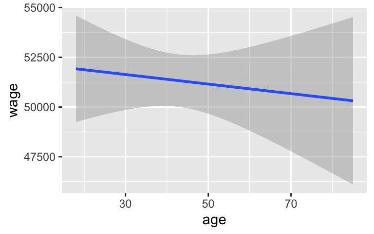

Let’s do this a bunch. Take 100 different shuffled samples and use each to estimate the model of wage by age (gray lines). These give us a sense of the sample models we’d expect IF H_0 were true. Is our sample estimate (blue line) consistent with H_0?

shuffled_models <- mosaic::do(100)*(
  CPS_2018 %>% 
    select(wage, age) %>% 
    sample_n(size = length(age), replace = TRUE) %>% 
    mutate(age = sample(age, size = length(age), replace = TRUE)) %>%
    with(lm(wage ~ age))
)

ggplot(CPS_2018, aes(x = age, y = wage)) + 
  geom_abline(data = shuffled_models, 
              aes(intercept = Intercept, slope = age), 
              color = "gray", size = 0.25) +
  geom_smooth(method = "lm", se = FALSE)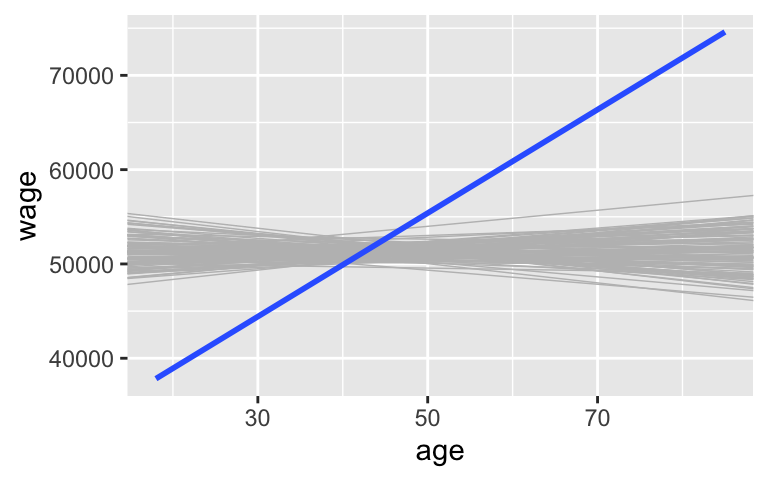

EXAMPLE 3: Step 2 – calculating & interpreting a test statistic

The sampling distribution below captures the range of age coefficient estimates we’d expect to see IF H_0 were true, i.e. IF the actual coefficient were 0. This is essentially the range of the slopes in our simulated model lines above, and is defined by the standard error of the age coefficient estimate:

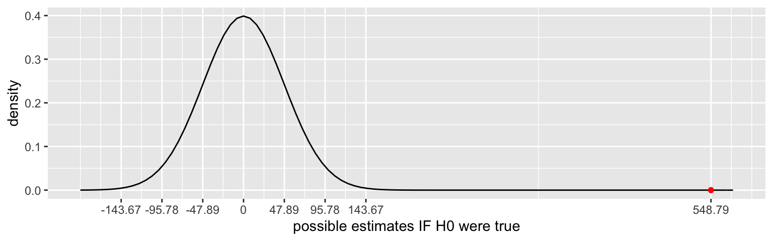
Our sample estimate of 548.79 is marked by the red dot. Its test statistic provides one measure of the compatibility of this estimate with H_0. Report the test statistic for our hypothesis test. For practice, both calculate this value “by hand” and find it in your model summary table.

coef(summary(wage_model_1))
##               Estimate Std. Error  t value     Pr(>|t|)
## (Intercept) 27954.3732 2146.56299 13.02285 1.862909e-38
## age           548.7934   47.89052 11.45933 3.258478e-30

Interpret the test statistic: Our estimate of the age coefficient is ___ standard errors above ___.

EXAMPLE 4: Step 2 – using a test statistic

What can we conclude from the test statistic?

Our sample data is not consistent with the null hypothesis that there’s no association between wage and age.
Our sample data is consistent with the null hypothesis that there’s no association between wage and age.

EXAMPLE 5: Step 2 – Calculate a p-value

The p-value provides another measure of the compatibility of our sample estimate with H_0. It’s the probability that we would have observed such a large coefficient estimate (548.79 or greater) IF in fact there were no association between wages and age (i.e. if H_0 were true).

Use the 68-95-99.7 Rule with the sketch from Example 3 to approximate the p-value:
- less than 0.0015
- between 0.0015 and 0.025
- bigger than 0.025
Calculate a more accurate p-value from the model summary(). Don’t forget to divide by 2!

coef(summary(wage_model_1))
##               Estimate Std. Error  t value     Pr(>|t|)
## (Intercept) 27954.3732 2146.56299 13.02285 1.862909e-38
## age           548.7934   47.89052 11.45933 3.258478e-30

EXAMPLE 6: Step 2 – Interpret the p-value

How can we interpret the p-value?

It’s very unlikely that we’d have observed such a steep increase in wages with age among our sample subjects “by chance”, i.e. if in fact there were no relationship between wages and age in the broader labor force.
In light of our sample data, it’s very unlikely that wages increase with age.
In light of our sample data, it’s very unlikely that wages and age are unrelated.

EXAMPLE 7: Step 3 – Conclusion

Finally, let’s pull it all together and make some conclusions about our hypotheses.

Based on the hypothesis test, is there a statistically significant association between wages and age? Explain.
Does this conclusion agree with the one we made using the confidence interval in Example 1?

EXAMPLE 8: Step 3 – A more nuanced conclusion

Statistical significance merely indicates that an association between wages and age exists. Consider an important follow-up question: is the magnitude of this association practically significant? That is, in the context of wages, is the scale of our coefficient estimate ($548.79 per year in age) large enough to be meaningful?

20.2 Exercises

In the next steps, we’ll explore the relationship between wages and marital status among 18–25 year olds. Let’s estimate this relationship using our sample data:

# Filter the data
CPS_2018_young <- CPS_2018 %>% 
  filter(age <= 25, wage < 200000)

# Model the relationship
wage_model_2 <- lm(wage ~ marital, data = CPS_2018_young)
coef(summary(wage_model_2))
##                Estimate Std. Error   t value     Pr(>|t|)
## (Intercept)   27399.471   1714.496 15.981066 1.849857e-52
## maritalsingle -6596.133   1817.411 -3.629412 2.955178e-04

# Plot the relationship
ggplot(CPS_2018_young, aes(y = wage, x = marital)) + 
  geom_boxplot()

Confidence interval
1. Calculate and interpret a 95% confidence interval for the maritalsingle coefficient. Hot tip: first interpret just the estimate to remind yourself what this coefficient is measuring.
2. Based on this interval, are you confident that on average, single workers have lower wages than married workers?

Hypotheses
A researcher states the following hypotheses about the (unknown) population maritalsingle coefficient $\beta_1$:

H_0: $\beta_1 = 0$
H_a: $\beta_1 < 0$

How can we interpret these hypotheses?
- H_0: There’s no association between wage and marital status.
  H_a: On average, wage decreases with marital status.
- H_0: There’s no association between wage and marital status.
  H_a: On average, wages are higher among single vs married workers.
- H_0: There’s no association between wage and marital status.
  H_a: On average, wages are lower among single vs married workers.

Test statistic
Report and interpret a test statistic for this hypothesis test.

coef(summary(wage_model_2))
##                Estimate Std. Error   t value     Pr(>|t|)
## (Intercept)   27399.471   1714.496 15.981066 1.849857e-52
## maritalsingle -6596.133   1817.411 -3.629412 2.955178e-04

p-value
1. Approximate a p-value for this hypothesis test using the 68-95-99.7 Rule:
  - less than 0.0015
  - between 0.0015 and 0.025
  - bigger than 0.025
2. Calculate a more accurate p-value from the model summary table.
```
coef(summary(wage_model_2))
##                Estimate Std. Error   t value     Pr(>|t|)
## (Intercept)   27399.471   1714.496 15.981066 1.849857e-52
## maritalsingle -6596.133   1817.411 -3.629412 2.955178e-04
```
3. Interpret this p-value.

Conclusion
What conclusion do you make about these hypotheses?
- Our sample data establishes that the typical wages among single workers are (statistically) significantly below those of married workers.
- Our sample data do not establish a significant association between wages and marital status.

PAUSE: We just did a “Two Sample t-Test”!

The hypothesis test above essentially compared two population means: the mean wage of single people and the mean wage of married people. This is known as a two sample t-test. “Two” sample because we’re comparing two means.

A hypothesis test for the intercept
We can also test hypotheses about model intercepts but, for reasons you’ll see here, these aren’t usually helpful. For example, in the population model $\text{wage} = \beta_0 + \beta_1\text{ maritalsingle}$ we can test:

H_0: $\beta_0 = 0$
H_a: $\beta_0 \ne 0$

We see in the model summary() below that the p-value for this hypothesis test is miniscule (1.85 * 10^(-52)):
```
coef(summary(wage_model_2))
##                Estimate Std. Error   t value     Pr(>|t|)
## (Intercept)   27399.471   1714.496 15.981066 1.849857e-52
## maritalsingle -6596.133   1817.411 -3.629412 2.955178e-04
```
Keeping in mind the meaning of the $\beta_0$ coefficient, what do you conclude?
- We have statistically significant evidence of a relationship between wages and marriage status.
- We have statistically significant evidence that there’s no relationship between wages and marriage status.
- We have statistically significant evidence that the average wage of single workers is non-0.
- We have statistically significant evidence that the average wage of married workers is non-0.

PAUSE: We just did a “One Sample t-Test”!

The hypothesis test above essentially compared one population mean (the mean wage of married people) to a hypothesized value (in this case, 0). This is a special case of a one sample t-test.

Controlling for age
Since we haven’t controlled for important covariates, we should be wary of using the above results to argue that there’s wage discrimination against single people. To this end, consider the relationship between wages and marriage status when controlling for age:

\[\text{wage} = \beta_0 + \beta_1\text{ maritalsingle} + \beta_2\text{ age}\]

Check out our sample estimate of this model:
```
wage_model_3 <- lm(wage ~ marital + age, data = CPS_2018_young)

# Model summary
coef(summary(wage_model_3))
##                 Estimate Std. Error    t value     Pr(>|t|)
## (Intercept)   -53547.003  5719.1332 -9.3627830 3.484809e-20
## maritalsingle  -1456.015  1714.3082 -0.8493312 3.958595e-01
## age             3483.197   236.4797 14.7293716 2.099717e-45

# Confidence intervals
confint(wage_model_3)
##                    2.5 %     97.5 %
## (Intercept)   -64767.154 -42326.852
## maritalsingle  -4819.252   1907.221
## age             3019.257   3947.138
```
What can we conclude from the 95% confidence interval for the marital single coefficient?
- Wage and marital status are significantly associated.
- Wage and marital status are not significantly associated (i.e. marital status is not a significant predictor of wage).
- When controlling for age, wage and marital status are significantly associated.
- When controlling for age, wage and marital status are not significantly associated (i.e. marital status is not a significant predictor of wage).

Testing hypotheses
Consider the following hypotheses about the maritalsingle coefficient in our model of wage by marital status and age:

H_0: $\beta_1 = 0$
H_a: $\beta_1 < 0$

How can we interpret these hypotheses?

H_0: When controlling for age, there’s no association between wages and marital status.
H_a: When controlling for age, single workers tend to have smaller wages than married workers.

H_0: There’s no association between wages and marital status.
H_a: Single workers tend to have smaller wages than married workers.

Testing the hypotheses

Report the test statistic and p-value for these hypotheses.

coef(summary(wage_model_3))
##                 Estimate Std. Error    t value     Pr(>|t|)
## (Intercept)   -53547.003  5719.1332 -9.3627830 3.484809e-20
## maritalsingle  -1456.015  1714.3082 -0.8493312 3.958595e-01
## age             3483.197   236.4797 14.7293716 2.099717e-45

What conclusion can we make from these results?

Reflection
Bringing it all together, what can we conclude about the relationship between wages and marital status from the combined results from wage_model_2 and wage_model_3?

Interaction?
In some cases, our research questions define what model we should construct. For example, we built wage_model_2 because we wanted to explore the relationship between wages and marital status while controlling for age. In other cases, hypothesis tests can aid the model building process. For example, should we have included an interaction term in wage_model_3? Build a new model and conduct a new hypothesis test that helps you answer this question.

20.3 Reflection

Hypothesis “t”-Tests for Model coefficients

Consider a population model of response variable $y$ by explanatory terms $x_1$, $x_2$, and $x_3$: \[y = \beta_0 + \beta_1x_1 + \beta_2x_2 + \beta_3x_3\] where population coefficients $\beta_0, \beta_1, \beta_2, \beta_3$ are unknown. Then the p-value given in the last column of the $x_1$ row in the model summary table corresponds to the following test:

\[\begin{split} H_0: & \; \beta_1 = 0 \\ H_a: & \; \beta_1 \ne 0 \\ \end{split}\]

In words:

$H_0$ represents “no $x_1$ effect”, i.e. when controlling for $x_2$ and $x_3$ there’s no significant relationship between $x_1$ and $y$.
$H_a$ represents an “$x_1$ effect”, i.e. even when controlling for $x_2$ and $x_3$ there’s a significant relationship between $x_1$ and $y$.

Note: We typically test a one-sided alternative $H_a: \beta_1 < 0$ or $H_a: \beta_1 > 0$. In this case, we divide the reported p-value by 2.

A Survey of Hypothesis Tests

Though we can use confidence intervals to answer such inferential questions, hypothesis tests provide a formal framework. There are countless types of hypothesis tests. The following are a few that we might see in the next few weeks. Though they differ in their goals, their structure is the same!

Test Name	Population quantities of interest	Example
t-tests for model coefficients	model coefficients	When controlling for job sector, is education associated with wage?
ANOVA	multiple model coefficients	With all categories combined, is job sector associated with wage?
one sample t-test	1 mean	Is the mean wage above $50,000?
two sample t-test	2 independent means	Is the mean wage higher for married vs single people?
ANOVA	2⁺ independent means
paired t-test	2 paired means	Is mean cholesterol pre-drug > mean post-drug?

20.4 Solutions