9 Covariates & multicollinearity
When you get to class
Install the palmerpenguins package. At right, click on the “Packages” tab, type palmerpenguins, and then click the install button.
Announcements
- Homework 3 is due Tuesday – it consists of the exercises in today’s activity and uses this Rmd template. I strongly encourage you to hand it in on Tuesday so that you can practice these concepts before the quiz.
- Quiz 1 is 1 week from today. Please see details on page 7 of the syllabus. I recommend that you review each activity and homework, trying to answer the questions without first looking at your notes.
9.1 Getting started
WHERE ARE WE
After today, we will have discussed all topics in exploratory analysis except interactions.

REVIEW
Interpret the coefficients in the below model of the time (in hours) that it takes to complete a hike by the hike’s length (in miles), vertical ascent(in feet), and rating (easy, moderate, or difficult).
library(ggplot2)
library(dplyr)
peaks <- read.csv("https://www.macalester.edu/~ajohns24/data/high_peaks.csv")

peaks_model <- lm(time ~ length + ascent + rating, data = peaks)
coef(summary(peaks_model))
##                    Estimate   Std. Error   t value     Pr(>|t|)
## (Intercept)     6.510651391 1.6298374041  3.994663 2.627176e-04
## length          0.459081885 0.0815831446  5.627166 1.465288e-06
## ascent          0.000187483 0.0003421535  0.547950 5.866973e-01
## ratingeasy     -3.168522397 0.8621911299 -3.674965 6.827232e-04
## ratingmoderate -2.476782718 0.6105855963 -4.056405 2.177589e-04
TODAY’S GOALS
Today’s exercises focus on multivariate model interpretation. Using the tools you already have, you’ll explore 2 nuances when building models with more than 1 predictor:
covariates
When exploring the relationship between response y and predictor x, there are often covariates (other predictors) for which we want to control. For example, in comparing the effectiveness of 2 different cold remedies, we might want to control for the age, general health, and severity of symptoms among the participants. We can control for these when conducting an experiment by creating 2 similar groups of subjects, and give 1 remedy to each. We need a different strategy when working with observational, not experimental, data.multicollinearity
When putting 2+ predictors into our model, we need to be mindful of the relationship among these predictors (not just their relationship with the response variable). When 2 predictors are strongly related, or multicollinear, it can impact the model interpretation and quality.
9.2 Exercises Part 1: Covariates
REMINDERS
- You will make mistakes throughout this activity. This is a natural part of learning any new language.
- We’re sitting in groups for a reason. Remember:
- You all have different experiences, both personal and academic.
- Be a good listener and be supportive when others make mistakes.
- Stay in sync with one another while respecting that everybody works at different paces.
- Don’t rush.
THE STORY
The CPS_2018 data set contains wage data collected by the Current Population Survey (CPS) in 2018. Using these data, we can explore the relationship between annual wages and marital status (married or single) among 18-34 year olds. The original codebook is here. These data reflect how the government collects data regarding employment.
# Load data
CPS_2018 <- read.csv("https://www.macalester.edu/~ajohns24/data/CPS_2018.csv")

# We'll focus on 18 to 34-year-olds that make under 250,000 dollars
CPS_2018 <- CPS_2018 %>%
  filter(age >= 18, age <= 34) %>%
  filter(wage < 250000)
Getting started
We’ll start with a small model ofwagevsmaritalstatus:# Visualize the relationship ggplot(CPS_2018, aes(y = wage, x = marital)) + geom_boxplot()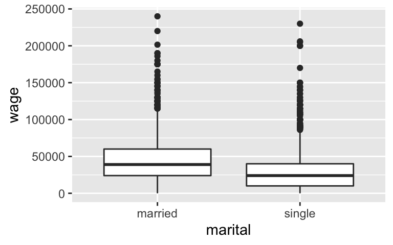
# Model the relationship CPS_model_1 <- lm(wage ~ marital, CPS_2018) coef(summary(CPS_model_1)) ## Estimate Std. Error t value Pr(>|t|) ## (Intercept) 46145.23 921.062 50.10002 0.000000e+00 ## maritalsingle -17052.37 1127.177 -15.12839 5.636068e-50- Interpret the
maritalsinglecoefficient, -17.052.37. - This model ignores important workplace covariates, thus we cannot use this coefficient as evidence of workplace inequity for single workers. Name at least 2 covariates for which we should control and explain your rationale.
- Interpret the
Controlling for age
Let’s start simple, by controlling for age (an imperfect measure of experience) in our model of wages by marital status. Unlike in the cold remedy example, we can’t assign people a marital status (that would be weird). Instead, we can control for age by putting it in our model! NOTE: Pause to think about the coefficients before answering the questions below.# Construct the model CPS_model_2 <- lm(wage ~ marital + age, CPS_2018) coef(summary(CPS_model_2)) ## Estimate Std. Error t value Pr(>|t|) ## (Intercept) -19595.948 3691.6998 -5.308110 1.184066e-07 ## maritalsingle -7500.146 1191.8526 -6.292847 3.545964e-10 ## age 2213.869 120.7701 18.331265 2.035782e-71Visualize this model by modifying the hint code. NOTE: Don’t get distracted by the last line. This is just making sure that the
geom_smoothmatches our model assumptions.# HINT CODE # ggplot(___, aes(y = ___, x = ___, color = ___)) + # geom____(size = 0.1, alpha = 0.5) + # geom_line(aes(y = CPS_model_2$fitted.values), size = 1.25)Suppose two workers are the same age, but one is married and the other is single. According to the model, by how much do we expect the single worker’s wage to differ from the married worker’s wage?
With your answer to part b in mind, which of the options below is another way to interpret the
maritalsinglecoefficient? On average…- Single workers make $7500 less than married workers.
- When controlling for (“holding constant”) age, single workers make $7500 less than married workers.
- Single workers make $7500 less than married workers.
Controlling for more covariates
We’ve seen that among all workers, the wage gap of single vs married workers is $17,052. We also saw that age accounts for some of this difference. Let’s see what happens when we control for even more workforce covariates: model wages by marital status while controlling forageand years ofeducation:CPS_model_3 <- lm(wage ~ marital + age + education, CPS_2018) coef(summary(CPS_model_3)) ## Estimate Std. Error t value Pr(>|t|) ## (Intercept) -64898.607 4099.8737 -15.829416 2.254709e-54 ## maritalsingle -6478.094 1119.9345 -5.784351 7.988760e-09 ## age 1676.796 116.3086 14.416777 1.102113e-45 ## education 4285.259 207.2158 20.680173 3.209448e-89Challenge: Add something to the code below to construct a single visualization of the relationship among these 4 variables (don’t delete anything). Mainly, start by visualizing wage vs age, and step by step incorporate information about marital status and education.
ggplot(CPS_2018, aes(x = age, y = wage)) +
  geom_point()
With so many variables, this is a tough model to visualize. If you had to draw it, how would the model trend appear: 1 point, 2 points, 2 lines, 1 plane, or 2 planes? Explain your rationale. Hot tip: pay attention to whether your predictors are quantitative or categorical.
Even if we can’t easily draw
CPS_model_3, the coefficients contain the information we want! How can we interpret the education coefficient? On average…- Wages increase by $4285 for every extra year of education.
- When controlling for marital status and age, wages increase by $4285 for every extra year of education.
- People with an education make $4285 more than those that don’t.
- Wages increase by $4285 for every extra year of education.
Which of the following is the best interpretation of the
maritalsinglecoefficient? On average…- When controlling for age and education, single workers make $6478 less than married workers.
- Single workers make $6478 less than married workers.
- When controlling for age and education, single workers make $6478 less than married workers.
Even more covariates
Let’s control for another workforce covariate: model wages by marital status while controlling forage(quantitative), years ofeducation(quantitative), and theindustryin which one works (categorical):CPS_model_4 <- lm(wage ~ marital + age + education + industry, CPS_2018) coef(summary(CPS_model_4)) ## Estimate Std. Error t value Pr(>|t|) ## (Intercept) -52498.857 7143.8481 -7.3488206 2.533275e-13 ## maritalsingle -5892.842 1105.6898 -5.3295615 1.053631e-07 ## age 1493.360 116.1673 12.8552586 6.651441e-37 ## education 3911.117 243.0192 16.0938565 4.500408e-56 ## industryconstruction 5659.082 6218.5649 0.9100302 3.628760e-01 ## industryinstallation_production 1865.650 6109.2613 0.3053806 7.600964e-01 ## industrymanagement 1476.884 6031.2901 0.2448704 8.065727e-01 ## industryservice -7930.403 5945.6509 -1.3338158 1.823603e-01 ## industrytransportation -1084.176 6197.2462 -0.1749448 8.611342e-01If we had to draw it, this model would appear as 12 planes. The original plane explains the relationship between wage and the 2 quantitative predictors, age and education. Then this plane is split into 12 (2*6) individual planes, 1 for each possible combination of marital status (2 possibilities) and industry (6 possibilities).
- When controlling for a worker’s age, marital status, and education, which industry tends to have the highest wages? The lowest? Provide some numerical evidence.
- Interpret the
maritalsinglecoefficient. NOTE: Don’t forget to “control for” the covariates in the model.
- OPTIONAL challenge: Construct a single visualization of the relationship among these 5 variables. Hot tip: utilize a
facet_wrap(~ ___).
- When controlling for a worker’s age, marital status, and education, which industry tends to have the highest wages? The lowest? Provide some numerical evidence.
- An even bigger model
Consider two people with the same age, education, industry, typical number of work hours, and health status. However, one is single and one is married.- Construct and use a new model to summarize the typical difference in the wages for these two people. Store this model as
CPS_model_5. - After controlling for all of these workforce covariates, do you still find the remaining wage gap for single vs married people to be meaningfully “large”? Can you think of any remaining factors that might explain part of this remaining gap? Or do you think we’ve found evidence of inequitable wage practices for single vs married workers?
- Construct and use a new model to summarize the typical difference in the wages for these two people. Store this model as
Model comparison & selection
Take two workers – one is married and the other is single. The models above provided the following insights into the typical difference in wages for these two groups:Model Assume the two people have the same… Wage difference R2 CPS_model_1NA -$17,052 0.067 CPS_model_2age -$7,500 0.157 CPS_model_3age, education -$6,478 0.257 CPS_model_4age, education, industry -$5,893 0.280 CPS_model_5age, education, industry, hours, health -$4,993 0.341 - Though this won’t always be the case in every analysis, notice that the
maritalcoefficient got closer and closer to 0 as we included more covariates in our model. Explain the significance of this phenomenon in the context of our analysis - what does it mean? - We’ve built several models here – and there are dozens more. Amongst so many options, it’s important to anchor our analysis and model building in our research goals. With respect to each possible goal below, explain which of our 5 models would be best. Make sure to provide some rationale.
- We want the strongest model of wages.
- We want to understand the relationship between wages and marital status, ignoring all other possible factors in wages.
- We want to understand the relationship between wages and marital status while controlling for a person’s age and education.
- We want to maximize our understanding of why wages vary from person to person while keeping our model as simple as possible.
- Consider goal iv. Why do you think simplicity can be a good model feature?
- Though this won’t always be the case in every analysis, notice that the
Data drill
NOTE: Come back to this exercise after class so that you can discuss the multicollinearity exercises with your group.Use
dplyrtools to complete the data drill below.# What is the median wage in each industry? # How many workers fall into each health group? # Obtain a dataset of workers aged 18 to 22 that are in good health # Show just the first 6 rows # Hint: <= is "less than or equal to" # Calculate the median age (in years) amongst workers in excellent health
9.3 Exercises Part 2: Multicollinearity
DIRECTIONS
In some of the exercises below, you’ll be asked to check in with your gut before checking your results. This is an important step in the learning process. These gut checks will be graded on completion, not correctness – you won’t be judged if your gut was wrong!
Multivariate models are great! We’ve seen that adding more predictors to a model increases R-squared (the strength of the model) and allows us to control for important covariates. BUT. We must also consider more nuances and limitations to indiscriminately adding more predictors to our model. To explore these ideas, load the following data on penguins:
# Load data
library(palmerpenguins)
data(penguins)
You can find a codebook for these data by typing ?penguins in your console (not Rmd). Our goal throughout will be to build a model of bill lengths (in mm):

(Art by @allison_horst)
To get started, the flipper_length_mm variable currently measures flipper length in mm. Let’s create and save a new variable named flipper_length_cm which measures flipper length in cm. NOTE: There are 10mm in a cm.
penguins <- penguins %>%
  mutate(flipper_length_cm = flipper_length_mm / 10)
Run the code chunk below to build a bunch of models that you’ll be exploring in the exercises:
penguin_model_1 <- lm(bill_length_mm ~ flipper_length_mm, penguins)
penguin_model_2 <- lm(bill_length_mm ~ flipper_length_cm, penguins)
penguin_model_3 <- lm(bill_length_mm ~ flipper_length_mm + flipper_length_cm, penguins)
penguin_model_4 <- lm(bill_length_mm ~ body_mass_g, penguins)
penguin_model_5 <- lm(bill_length_mm ~ flipper_length_mm + body_mass_g, penguins)
Modeling bill length by flipper length
What can a penguin’s flipper (arm) length tell us about their bill length? To answer this question, we’ll consider 3 of our models:model predictors penguin_model_1flipper_length_mmpenguin_model_2flipper_length_cmpenguin_model_3flipper_length_mm + flipper_length_cmPlots of the first two models are below:
ggplot(penguins, aes(y = bill_length_mm, x = flipper_length_mm)) +
  geom_point() +
  geom_smooth(method = "lm", se = FALSE)
ggplot(penguins, aes(y = bill_length_mm, x = flipper_length_cm)) +
  geom_point() +
  geom_smooth(method = "lm", se = FALSE)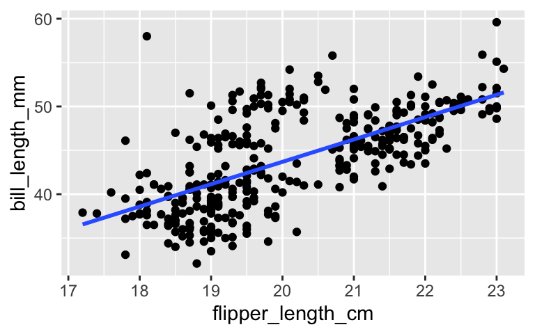
Before examining the model summaries, ask your gut: Do you think the
penguin_model_2R-squared will be less than, equal to, or more than that ofpenguin_model_1? Similarly, how do you think thepenguin_model_3R-squared will compare to that ofpenguin_model_1?
Check your gut: Examine the R-squared values for the three penguin models and summarize how these compare.
summary(penguin_model_1)$r.squared
## [1] 0.430574
summary(penguin_model_2)$r.squared
## [1] 0.430574
summary(penguin_model_3)$r.squared
## [1] 0.430574
Explain why your observation in part b makes sense. Support your reasoning with a plot of just the 2 predictors:
flipper_length_mmvsflipper_length_cm.OPTIONAL challenge: In
summary(penguin_model_3), theflipper_length_cmcoefficient isNA. Explain why this makes sense. HINT: Thinking about what you learned about controlling for covariates, why wouldn’t it make sense to interpret this coefficient? BONUS: For those of you that have taken MATH 236, this has to do with matrices that are not of full rank!
Incorporating
body_mass_g
In this exercise you’ll consider 3 models ofbill_length_mm:model predictors penguin_model_1flipper_length_mmpenguin_model_4body_mass_gpenguin_model_5flipper_length_mm + body_mass_g- Which is the better predictor of
bill_length_mm:flipper_length_mmorbody_mass_g? Provide some numerical evidence. penguin_model_5incorporates bothflipper_length_mmandbody_mass_gas predictors. Before examining a model summary, ask your gut: Will thepenguin_model_5R-squared be close to 0.35, close to 0.43, or greater than 0.6?- Check your intuition. Report the
penguin_model_5R-squared and summarize how this compares to that ofpenguin_model_1andpenguin_model_4. - Explain why your observation in part c makes sense. Support your reasoning with a plot of the 2 predictors:
flipper_length_mmvsbody_mass_g.
- Which is the better predictor of
Redundancy & Multicollinearity
The exercises above have illustrated special phenomena in multivariate modeling:- two predictors are redundant if they contain the same exact information
- two predictors are multicollinear if they are strongly associated (they contain very similar information) but are not completely redundant.
And as a reminder, we checked out 5 models:
model predictors penguin_model_1flipper_length_mmpenguin_model_2flipper_length_cmpenguin_model_3flipper_length_mm + flipper_length_cmpenguin_model_4body_mass_gpenguin_model_5flipper_length_mm + body_mass_g- Which model had redundant predictors and which predictors were these?
- Which model had multicollinear predictors and which predictors were these?
- In general, what happens to the R-squared value if we add a redundant predictor into a model: will it decrease, stay the same, increase by a small amount, or increase by a significant amount?
- Similarly, what happens to the R-squared value if we add a multicollinear predictor into a model: will it decrease, stay the same, increase by a small amount, or increase by a significant amount?
- Model selection & curiosity
- There are so many models we could build! Which predictors would you include in your model if you wanted to understand the relationship between bill length and depth when controlling for penguin species?
- Which predictors would you include in your model if you wanted to be able to predict a penguin’s bill length from its flipper length alone (because maybe penguins let us get closer to their arms than their nose?)?
- Aren’t you so curious about penguins? Identify one new question of interest, and explore this question using the data. It can be a simple question and answered in 1 line / 1 set of lines / 1 plot of R code, so long as it’s not explored elsewhere in this activity.
9.4 Solutions
There are no solutions to this activity since the exercises are due as Homework 3.