4 Modeling bivariate relationships: Part 1
When you get to class
Open today’s Rmd file linked on the day-to-day schedule. Name and save the file.
Do not knit until the end. The chunks in this Rmd are meant to be run and examined one at a time!
For reference, you might open the slides for today’s preparatory video here.
Announcements
- As usual, there is a video and checkpoint to complete before Thursday’s class.
- Homework 1 is due next Tuesday at 930am. Hot tips:
- Start early
This is not designed to complete in one sitting. So that you have ample time to explore and ask questions, I recommend that you start the homework today.
- Review
Be sure to review the course material before diving into the homework. You’ll learn more and homework will be less bumpy.
- Start early
4.1 Review
In today’s activity, we’ll explore the Capital Bikeshare data:
# Load packages & import data
library(ggplot2)
library(dplyr)
bikes <- read.csv("https://www.macalester.edu/~dshuman1/data/155/bike_share.csv")
We should always start by just getting to know our data:
# How much data do we have?
dim(bikes)
## [1] 731  15

# What does the data look like?
head(bikes, 3)
##         date season year month day_of_week weekend holiday temp_actual
## 1 2011-01-01 winter 2011   Jan         Sat    TRUE      no    57.39952
## 2 2011-01-02 winter 2011   Jan         Sun    TRUE      no    58.82468
## 3 2011-01-03 winter 2011   Jan         Mon   FALSE      no    46.49166
##   temp_feel humidity windspeed weather_cat riders_casual riders_registered
## 1  64.72625 0.805833  10.74988      categ2           331               654
## 2  63.83651 0.696087  16.65211      categ2           131               670
## 3  49.04645 0.437273  16.63670      categ1           120              1229
##   riders_total
## 1          985
## 2          801
## 3         1349
Our main goal will be to explore daily ridership among registered users, as measured by riders_registered. Let’s start by getting to know this variable. In your code, pay special attention to formatting / readability (just as you would in writing a paper): use spaces, tab subsequent lines, use comments, etc.
# Construct a plot of riders_registered


# Calculate the typical number of riders per day
4.2 Getting started
GOAL
Now that we have a sense for the data we’re working with and some univariate patterns, we can start to explore: in our sample data, what’s the RELATIONSHIP between two different variables? For example, what’s the relationship between ridership and temperature?
Statistical modeling
We can summarize relationships among 2 variables using a statistical model. Let
\(y\) = a quantitative response variable
\(x\) = a predictor of \(y\) (we’ll assume for now that \(x\) is quantitative)
Then a linear regression model describes the typical relationship between \(y\) and \(x\):
\[y = \beta_0 + \beta_1 x\]
where
\(\beta_0\) (“beta 0”) is the y-intercept. It describes the typical value of \(y\) when \(x\) is 0, ie. where the model line crosses the y-axis.
\(\beta_1\) (“beta 1”) is the slope. It describes the typical change in \(y\) per 1-unit increase in \(x\).
Least squares estimation
We can’t actually know the exact model, but can estimate it using our sample data:
\[y = \hat{\beta}_0 + \hat{\beta}_1 x\]
where we calculate the sample estimates \(\hat{\beta}_0\) and \(\hat{\beta}_1\) using the least squares method. Specifically, let
- \(\hat{y}\) = the model predicted value of \(y\)
- \(y - \hat{y}\) = the residual, i.e. distance between the observed and predicted value of \(y\) (which we want to be small)
Then \(\hat{\beta}_0\) and \(\hat{\beta}_1\) minimize the overall size of the residuals:
\[\text{sum of squared residuals} = \sum (y - \hat{y})^2\]

4.3 Exercises
Goals
Practice building and interpreting plots and models of bivariate relationships.
In the first exercises, you’ll re-construct the model and plots you saw in today’s video. You’ll subsequently extend these tools to new settings.
Recall that software helps us do statistics. In today’s code, you might often ask yourself: “what does this part do?”. The best way to answer this question is to play around – if you remove or change that part of the code, what happens?!
Reminders
You will make mistakes throughout this activity. This is a natural part of learning any new language.
We’re sitting in groups for a reason. Remember:
- You all have different experiences, both personal and academic.
- Be a good listener and be supportive when others make mistakes.
- Stay in sync with one another while respecting that everybody works at different paces.
- Don’t rush.
If you don’t finish the activity during class, you are expected to complete it outside of class. To this end, remember that there are solutions in the online manual.
- Hello!
Introduce yourselves and share your dream breakfast.
Constructing scatterplots
In these first exercises, we’ll explore the relationship betweenriders_registeredandtemp_feel. Separately run each chunk below and add a comment (#) about what you see. The goal isn’t to memorize the code but to start observing patterns in how the code works.# ??? ggplot(bikes, aes(x = temp_feel, y = riders_registered))# ??? ggplot(bikes, aes(x = temp_feel, y = riders_registered)) + geom_point()# ??? ggplot(bikes, aes(x = temp_feel, y = riders_registered)) + geom_point() + geom_smooth(method = "lm", se = FALSE)
Modeling trend: Part 1
The scatterplot ofriders_registeredvstemp_feelexhibits the trend in this relationship as well as the degree to which districts vary from this trend. The linear regression trend line is drawn in your scatterplot above. Let’s dig into the details. Chunk by chunk, take note of the syntax:# Construct and save the model as bike_model_1 # What's the purpose of "riders_registered ~ temp_feel"??? # What's the purpose of "data = bikes"??? bike_model_1 <- lm(riders_registered ~ temp_feel, data = bikes)# A long summary of the model stored in bike_model_1 summary(bike_model_1)# A simplified model summary coef(summary(bike_model_1))
Modeling trend: Part 2
Focus on the simplified model summary. Use this information to write out a formula for the linear trend exhibited in the scatterplot above. (This should be similar to the formula you saw on the video!)riders_registered = ___ + ___ temp_feelRECALL: Since we didn’t observe any temperatures near 0, it doesn’t make sense to interpret the intercept (-667.916) – it simply summarizes where the linear trend “lives”. Further, the
temp_feelcoefficient (57.892) indicates that, on average, for every extra 1 degree increase in temperature, we expect nearly 58 more riders.
Predictions & residuals
On August 17, 2012, thetemp_feelwas 53.816 degrees and there were 5665 riders. We can get data for this day using thefilter()andselect()dplyrfunctions. Note, but don’t worry about the syntax – we haven’t learned this yet:bikes %>% filter(date == "2012-08-17") %>% select(riders_registered, temp_feel) ## riders_registered temp_feel ## 1 5665 53.816Peak back at the scatterplot. Identify which point corresponds to August 17, 2012. Is it close to the trend? Were there more riders than expected or fewer than expected?
Use your model formula from the previous exercise to predict the ridership on August 17, 2012 from the temperature on that day. (That is, where do days with this temperature fall on the model trend line?)
Check your part b calculation using the
predict()function. Take careful note of the syntax – it’s a bit tedious.predict(bike_model_1, newdata = data.frame(temp_feel = 53.816))Calculate the residual or prediction error. How far does the observed ridership fall from the model prediction?
residual = observed y - predicted y = ???
- Interpreting residuals
- Are days with positive residuals above or below the trend?
- Does this mean that the model over- or under-estimates ridership on these days?
- Are days with negative residuals above or below the trend?
- Does this mean that the model over- or under-estimates ridership on these days?
Your turn: windspeed
Let’s turn our attention to the relationship betweenriders_registeredandwindspeed.# Construct a visualization of this relationship # Include a representation of the relationship trend # Use lm to construct a model of riders_registered vs windspeed # Save this as bike_model_2 # Get a short summary of this model
- Interpreting the results
- Summarize your observations from the visualizations.
- Write out a formula for the model trend.
- Interpret both the intercept and the windspeed coefficient. THINK: What does a negative slope indicate?
- Use this model to predict the ridership on August 17, 2012 and calculate the corresponding residual. HINT: You’ll first need to find the windspeed on this date!
- Clean, knit, and save your work!
4.4 More exercises: data drill
The exercises below are designed to help you keep building your dplyr skills. These skills are important to data cleaning and digging, which in turn is important to really making meaning of our data. We’ll work with a simpler set of 10 data points:
new_bikes <- bikes %>%
  select(date, temp_feel, humidity, riders_registered, day_of_week) %>%
  head(10)
verb 1: summarize
Thus far, in thedplyrgrammar you’ve seen 3 verbs or action words:summarize(),select(),filter(). Try out the following code and then summarize the point of thesummarize()function:new_bikes %>% summarize(mean(temp_feel), mean(humidity))
verb 2: select
Try out the following code and then summarize the point of theselect()function:new_bikes %>% select(date, temp_feel)new_bikes %>% select(-date, -temp_feel)
verb 3: filter
Try out the following code and then summarize the point of thefilter()function:new_bikes %>% filter(riders_registered > 850)new_bikes %>% filter(day_of_week == "Sat")new_bikes %>% filter(riders_registered > 850, day_of_week == "Sat")
Your turn
Usedplyrverbs to complete each task below.# Keep only information about the humidity and day of week # Keep only information about the humidity and day of week using a different approach # Keep only information for Sundays # Keep only information for Sundays with temperatures below 50 # Calculate the maximum and minimum temperatures
4.5 Solutions
- .
.
# Set up the canvase
ggplot(bikes, aes(x = temp_feel, y = riders_registered))
# Add points
ggplot(bikes, aes(x = temp_feel, y = riders_registered)) +
  geom_point()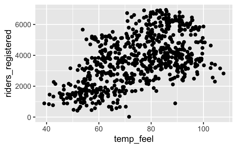
# Add regression line
ggplot(bikes, aes(x = temp_feel, y = riders_registered)) +
  geom_point() +
  geom_smooth(method = "lm", se = FALSE)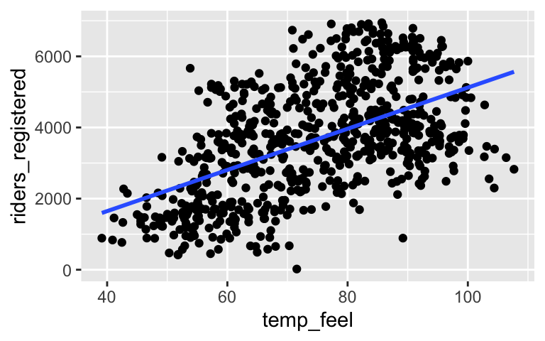
.
# Construct and save the model as bike_model_1
# The first part indicates what relationship we're interested in.
# The second part indicates what data we're using to learn about this relationship
bike_model_1 <- lm(riders_registered ~ temp_feel, data = bikes)

# A long summary of the model stored in bike_model_1
summary(bike_model_1)
##
## Call:
## lm(formula = riders_registered ~ temp_feel, data = bikes)
##
## Residuals:
##     Min      1Q  Median      3Q     Max
## -3607.1  -959.2  -153.8   998.2  3304.8
##
## Coefficients:
##             Estimate Std. Error t value Pr(>|t|)
## (Intercept) -667.916    251.608  -2.655  0.00811 **
## temp_feel     57.892      3.306  17.514  < 2e-16 ***
## ---
## Signif. codes:  0 '***' 0.001 '**' 0.01 '*' 0.05 '.' 0.1 ' ' 1
##
## Residual standard error: 1310 on 729 degrees of freedom
## Multiple R-squared:  0.2961, Adjusted R-squared:  0.2952
## F-statistic: 306.7 on 1 and 729 DF,  p-value: < 2.2e-16

# A simplified model summary
coef(summary(bike_model_1))
##               Estimate Std. Error   t value     Pr(>|t|)
## (Intercept) -667.91568 251.608155 -2.654587 8.113787e-03
## temp_feel     57.89236   3.305577 17.513543 1.383488e-57
- riders_registered = -667.91568 + 57.89236 temp_feel
- .
It’s the lonely point toward the top left - far from the trend.
riders_registered = -667.91568 + 57.89236*53.816 = 2447.62
.
predict(bike_model_1, newdata = data.frame(temp_feel = 53.816))
##       1
## 2447.62
residual = 5665 - 2447.62 = 3217.38
- .
- above (observed > predicted)
- under-estimates
- below (observed < predicted)
- over–estimates
.
# Construct a visualization of this relationship
# Include a representation of the relationship trend
ggplot(bikes, aes(x = windspeed, y = riders_registered)) +
  geom_point() +
  geom_smooth(method = "lm", se = FALSE)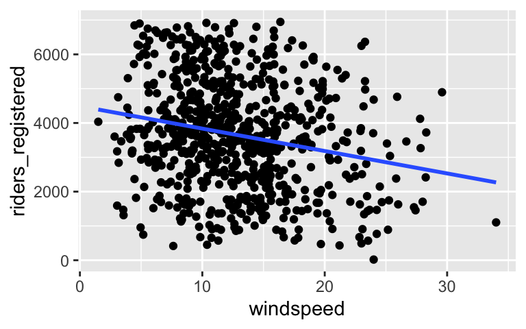
# Use lm to construct a model of riders_registered vs windspeed
# Save this as bike_model_2
bike_model_2 <- lm(riders_registered ~ windspeed, data = bikes)

# Get a short summary of this model
coef(summary(bike_model_2))
##               Estimate Std. Error   t value      Pr(>|t|)
## (Intercept) 4490.09761  149.65992 30.002005 2.023179e-129
## windspeed    -65.34145   10.86299 -6.015053  2.844453e-09
- Interpreting the results
There’s a weak, negative relationship – ridership tends to be smaller on windier days.
riders_registered = 4490.09761 - 65.34145 windspeed.
On days with no wind, we’d expect around 4490 riders. (0 is a little beyond what we observed, but not by much!) And for every 1mph increase in windspeed, we expect ridership to decrease by 65 riders on average.
.
bikes %>%
  filter(date == "2012-08-17") %>%
  select(riders_registered, windspeed)
##   riders_registered windspeed
## 1              5665  15.50072

# prediction
4490.09761 - 65.34145 * 15.50072
## [1] 3477.258

# residual
5665 - 3477.258
## [1] 2187.742
- .
summarize()calculates numerical summaries of variables (columns)new_bikes <- bikes %>% select(date, temp_feel, humidity, riders_registered, day_of_week) %>% head(10) new_bikes %>% summarize(mean(temp_feel), mean(humidity)) ## mean(temp_feel) mean(humidity) ## 1 51.97573 0.5436459
select()selects variables (columns)new_bikes %>% select(date, temp_feel) ## date temp_feel ## 1 2011-01-01 64.72625 ## 2 2011-01-02 63.83651 ## 3 2011-01-03 49.04645 ## 4 2011-01-04 51.09098 ## 5 2011-01-05 52.63430 ## 6 2011-01-06 52.98881 ## 7 2011-01-07 50.79551 ## 8 2011-01-08 46.60286 ## 9 2011-01-09 42.45575 ## 10 2011-01-10 45.57992 new_bikes %>% select(-date, -temp_feel) ## humidity riders_registered day_of_week ## 1 0.805833 654 Sat ## 2 0.696087 670 Sun ## 3 0.437273 1229 Mon ## 4 0.590435 1454 Tue ## 5 0.436957 1518 Wed ## 6 0.518261 1518 Thu ## 7 0.498696 1362 Fri ## 8 0.535833 891 Sat ## 9 0.434167 768 Sun ## 10 0.482917 1280 Mon
filter()keeps only days (rows) that meet the given condition(s)new_bikes %>% filter(riders_registered > 850) ## date temp_feel humidity riders_registered day_of_week ## 1 2011-01-03 49.04645 0.437273 1229 Mon ## 2 2011-01-04 51.09098 0.590435 1454 Tue ## 3 2011-01-05 52.63430 0.436957 1518 Wed ## 4 2011-01-06 52.98881 0.518261 1518 Thu ## 5 2011-01-07 50.79551 0.498696 1362 Fri ## 6 2011-01-08 46.60286 0.535833 891 Sat ## 7 2011-01-10 45.57992 0.482917 1280 Mon new_bikes %>% filter(day_of_week == "Sat") ## date temp_feel humidity riders_registered day_of_week ## 1 2011-01-01 64.72625 0.805833 654 Sat ## 2 2011-01-08 46.60286 0.535833 891 Sat new_bikes %>% filter(riders_registered > 850, day_of_week == "Sat") ## date temp_feel humidity riders_registered day_of_week ## 1 2011-01-08 46.60286 0.535833 891 Sat
.
# Keep only information about the humidity and day of week
new_bikes %>%
  select(humidity, day_of_week)
##    humidity day_of_week
## 1  0.805833         Sat
## 2  0.696087         Sun
## 3  0.437273         Mon
## 4  0.590435         Tue
## 5  0.436957         Wed
## 6  0.518261         Thu
## 7  0.498696         Fri
## 8  0.535833         Sat
## 9  0.434167         Sun
## 10 0.482917         Mon

# Keep only information about the humidity and day of week using a different approach
new_bikes %>%
  select(-date, -temp_feel, -riders_registered)
##    humidity day_of_week
## 1  0.805833         Sat
## 2  0.696087         Sun
## 3  0.437273         Mon
## 4  0.590435         Tue
## 5  0.436957         Wed
## 6  0.518261         Thu
## 7  0.498696         Fri
## 8  0.535833         Sat
## 9  0.434167         Sun
## 10 0.482917         Mon


# Keep only information for Sundays
new_bikes %>%
  filter(day_of_week == "Sun")
##         date temp_feel humidity riders_registered day_of_week
## 1 2011-01-02  63.83651 0.696087               670         Sun
## 2 2011-01-09  42.45575 0.434167               768         Sun

# Keep only information for Sundays with temperatures below 50
new_bikes %>%
  filter(day_of_week == "Sun", temp_feel < 50)
##         date temp_feel humidity riders_registered day_of_week
## 1 2011-01-09  42.45575 0.434167               768         Sun

# Calculate the maximum and minimum temperatures
new_bikes %>%
  summarize(min(temp_feel), max(temp_feel))
##   min(temp_feel) max(temp_feel)
## 1       42.45575       64.72625