18 Confidence intervals
Announcements
- Homework 6 is due Thursday by 930am.
- Checkpoint 15 is due Thursday by 930am.
- Mini-project phase 1 is due next Tuesday, one week from today. There will be time to work on this in class on Thursday, and possibly toward the end of class today. Collaboration both inside and outside class is a critical aspect of the project outcome and assessment, so please use this time :)
18.1 Getting started
Where are we?
What conclusions can we make about the broader population of interest using data on just a sample?! To answer this question we must understand and communicate the potential error in our sample estimates.
Recall
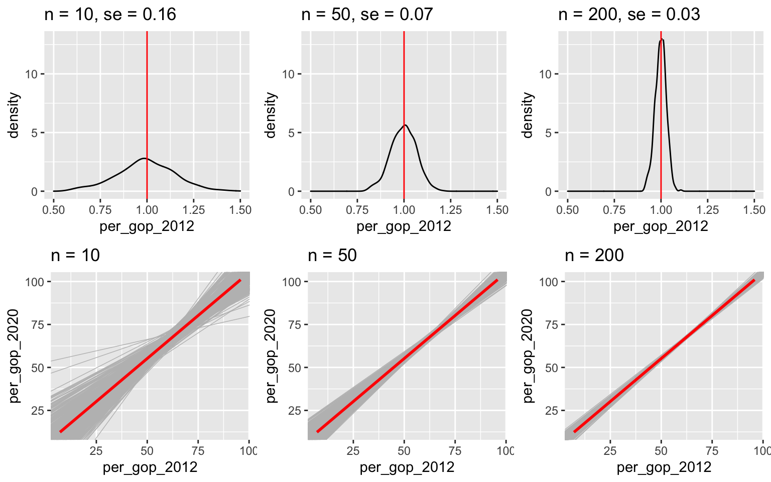
Using election data on the full population of U.S. counties (minus Alaska), the “actual” model between the 2020 and 2012 Republican support is as follows:
\[\text{per_gop_2020} = \beta_0 + \beta_1 \text{ per_gop_2012} = 5.179 + 1.000 \text{ per_gop_2012}\]
# Load packages
library(dplyr)
library(ggplot2)
library(mosaic)

# Import & wrangle data
elections <- read.csv("https://www.macalester.edu/~ajohns24/data/election_2020.csv") %>%
  mutate(per_gop_2020 = 100*per_gop_2020,
         per_gop_2012 = 100*per_gop_2012)

# Build and summarize the model
population_mod <- lm(per_gop_2020 ~ per_gop_2012, data = elections)
coef(summary(population_mod))
##              Estimate  Std. Error   t value     Pr(>|t|)
## (Intercept)  5.179393 0.486313057  10.65033 4.860116e-26
## per_gop_2012 1.000235 0.007896805 126.66328 0.000000e+00
Yet, suppose we were only able to sample n of these counties. In the previous activity, we simulated the corresponding sampling distributions and standard errors for the slope estimates \(\hat{\beta}_1\) by taking 500 different samples of size n. Recall:
The standard error measures the typical or standard error in the \(\hat{\beta}_1\) estimates.
For example, for samples of size 50, the slope estimates tend to be off by 0.07 units.
Standard error decreases as sample size increases. That is, the more data have, the closer our estimates tend to be to the actual values we’re estimating.
Central Limit Theorem (CLT)
So long as our sample size n is “large enough”, the possible sample estimates \(\hat{\beta}\) of some population feature \(\beta\) are Normally distributed around \(\beta\) with some standard error:
\[\hat{\beta} \sim N(\beta, \text{standard error}^2)\]
Thus by the 68-95-99.7 Rule:
- 68% of samples will produce \(\hat{\beta}\) estimates within 1 st. err. of \(\beta\)
- 95% of samples will produce \(\hat{\beta}\) estimates within 2 st. err. of \(\beta\)
- 99.7% of samples will produce \(\hat{\beta}\) estimates within 3 st. err. of \(\beta\)

Confidence intervals
To communicate and contextualize the potential error in \(\hat{\beta}\), we can calculate a confidence interval for \(\beta\). This:
- reflects the error in our estimate \(\hat{\beta}\); while
- providing a range of plausible values for \(\beta\); thus
- allows us to draw fair conclusions about the population using data from our sample!
Using the Central Limit Theorem, an approximate 95% confidence interval for \(\beta\) can be calculated by:
\[\hat{\beta} \pm 2 \text{ standard errors}\]
More precise calculations are provided in RStudio.
18.2 Exercises
Goals
Dig into some more details about building, interpreting, and utilizing confidence intervals.
Directions
Run this chunk to define a function that’s designed for this activity:
CI_plot <- function(level, n){
  # Take 100 samples of size n
  # Calculate confidence intervals from each sample

  CIs <- mosaic::do(100)*(
    elections %>%
      sample_n(size = n, replace = FALSE) %>%
      with(confint(lm(per_gop_2020 ~ per_gop_2012, data = .), level = level)) %>%
      as.data.frame() %>%
      tail(1)
  )
  CIs <- CIs %>%
    select(4, 1, 2)
  names(CIs) <- c("sample", "lower", "upper")
  CIs <- CIs %>%
    mutate(lucky = (lower < 1.000 & upper > 1.000),
           estimate = (upper + lower) / 2) %>%
    select(1, 5, 2:4)

  ggplot(CIs, aes(y = sample, x = lower, color = lucky)) +
    geom_segment(aes(x = lower, xend = upper, y = sample, yend = sample)) +
    geom_point(aes(x = estimate, y = sample)) +
    lims(x = c(0.55, 1.45)) +
    geom_vline(xintercept = 1.000) +
    scale_color_manual(values = c("red", "black")) +
    ggtitle(paste0("confidence = ", level*100, "%, n = ", n))
}
18.2.1 Part 1: Constructing & interpreting CIs
- Hello!
When 70 degree spring weather finally comes, what’s the first thing you’ll do?
Build a sample model
Let’s pretend we don’t have access to the full population. Instead, take one sample of 50 counties:# Take a sample set.seed(34) one_sample_50 <- sample_n(elections, size = 50, replace = FALSE)And then use this sample to estimate the model:
# Estimate the model one_sample_model <- lm(per_gop_2020 ~ per_gop_2012, one_sample_50) # Check it out coef(summary(one_sample_model)) ## Estimate Std. Error t value Pr(>|t|) ## (Intercept) 11.8822173 3.26519505 3.639053 6.680168e-04 ## per_gop_2012 0.8963895 0.05152905 17.395809 2.309632e-22What’s your sample estimate of the
per_gop_2012coefficient? How close is this to the actual population value of 1.000?What’s the standard error of this estimate? NOTE: This is estimated from our data using a formula that utilizes linear algebra.
The standard error from part b is a mere approximation of the typical error in a slope estimate, calculated from our one sample. Based on 500 different samples of size 50, our simulation suggested that the actual standard error is around 0.07. How close was your estimate from part b? Does it overestimate or underestimate the potential error in the
per_gop_2012estimate? NOTE: The point here is that in taking a leap from the sample to the population, nothing is perfect!
Applying the CLT
Based on theone_sample_50data alone, the CLT assumes that the possible sample estimates of theper_gop_2012coefficient, \(\hat{\beta}_1\), vary from sample to sample, are Normally centered around the actual population coefficient \(\beta_1\), and have a typical error of 0.0515:\[\hat{\beta}_1 \stackrel{\cdot}{\sim} N\left(\beta_1, 0.0515^2\right)\]
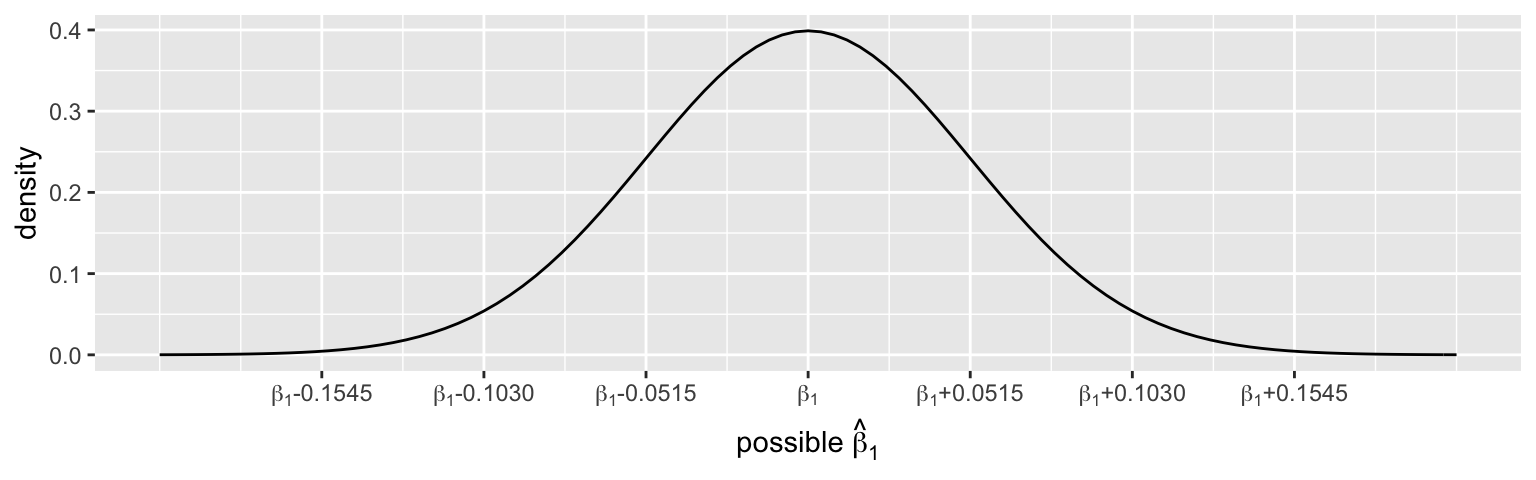
According to the CLT, approximately what % of samples will produce estimates \(\hat{\beta}_1\) that are…
- bigger than \(\beta_1\)
- lucky: within 2 standard errors (0.1030) of \(\beta_1\)
- unlucky: more than 2 standard errors (0.1030) from \(\beta_1\)
- really unlucky: more than 3 standard errors (0.1545) from \(\beta_1\)
- bigger than \(\beta_1\)
Using the CLT to construct a 95% confidence interval
Recall our sample model results:coef(summary(one_sample_model)) ## Estimate Std. Error t value Pr(>|t|) ## (Intercept) 11.8822173 3.26519505 3.639053 6.680168e-04 ## per_gop_2012 0.8963895 0.05152905 17.395809 2.309632e-22Use these results to calculate a 95% confidence interval for the actual population coefficient \(\beta_1\).
The 68-95-99.7 Rule is just a handy but rough guide. We can calculate a more accurate confidence interval in RStudio. (Was your approximation from part a close?)
confint(one_sample_model, level = 0.95)
- Were we lucky?
Did our sample produce a 95% confidence interval that contains the actual \(\beta_1 = 1.000\) value? Thus is ourone_sample_50one of the lucky samples? NOTE: If not, it’s not because we did anything wrong! It’s just an unlucky roll of the dice.
95% confidence
The use of “95% confidence” (instead of 100% confidence) indicates that such unlucky samples are possible. But what exactly does “95% confidence” mean? To answer this question, let’s repeat our experiment 100 times. Using the function below we can:- Take 100 different samples of 50 counties each.
- From each sample, calculate a 95% CI for \(\beta_1\).
- Then plot the 100 CIs. Each sample’s interval is centered at its estimate \(\hat{\beta}_1\), represented by a dot. Intervals that do NOT cover the true \(\beta_1 = 1.000\) are highlighted in red.
set.seed(1) CI_plot(level = 0.95, n = 50)QUESTION: What percentage of your 100 intervals do cover \(\beta_1\)? Not coincidentally, this should be close to 95%!
Impact of sample size
Suppose we increase our sample size from 50 to 200 counties. What does your intuition say: will the 95% confidence intervals for \(\beta_1\) be narrower or wider?
Check your intuition:
set.seed(1) CI_plot(level = 0.95, n = 200)Approximately what % of the 95% CIs contain \(\beta_1\)?
Impact of confidence level
Consider lowering our confidence level from 95% to 68% so that only 68% of samples would produce 68% CIs that cover \(\beta_1\). Intuitively, if we’re only 68% confident in a 68% CI, will it be narrower or wider than a 95% CI?
If we calculate an approximate 95% CI for \(\beta_1\) by \(\hat{\beta}_1\) +/- 2 standard errors, how would we calculate a 68% CI?
Check your intuition.
# FIRST: For a point of comparison, re-examine the 95% CIs for samples of size 50 CI_plot(level = 0.95, n = 50)# THEN: Check out 68% CIs for samples of size 50 set.seed(1) CI_plot(level = 0.68, n = 50)What if we wanted to be VERY confident that our CI covered \(\beta_1\)? Check out 100 different 99.7% CIs for \(\beta_1\):
set.seed(1) CI_plot(level = 0.997, n = 50)Or if we wanted to be 100% confident! Note that these lines actually go on forever, from negative to positive infinity:
CI_plot(level = 1, n = 50)
Trade-offs
Summarize the trade-offs in increasing confidence levels:
- As confidence level increases, does the percent of CIs that cover the actual population value increase, decrease, or stay the same?
- As confidence level increases, does the width of a CI increase, decrease, or stay the same?
- Why is a very wide CI less useful than a narrower CI?
- As confidence level increases, does the percent of CIs that cover the actual population value increase, decrease, or stay the same?
- Traditions
Practitioners typically use a 95% confidence level. Comment on why you think this is.
18.2.2 Part 2: Utilizing CIs for inference
Now that we know how to construct and interpret confidence intervals, let’s use them to make inferences about the broader population! For the next exercises, we’ll use the high_peaks data on hiking trails in the 46 “high peaks” in the Adirondack mountains of northern New York state. Our goal will be to understand whether the time it takes to complete each hike is significantly associated with various features: a hike’s highest elevation, length, and difficulty rating.
time versus length – part 1
Load the data, then use this to visualize and model the relationship between a hike’s completion time (in hours) and length (in miles).peaks <- read.csv("https://www.macalester.edu/~ajohns24/data/high_peaks.csv") # Visualize the relationship ggplot(peaks, aes(y = time, x = length)) + geom_point() + geom_smooth(method = "lm", se = FALSE)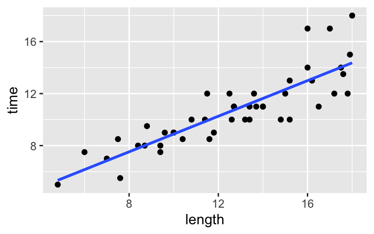
# Model the relationship model_1 <- lm(time ~ length, data = peaks) coef(summary(model_1)) ## Estimate Std. Error t value Pr(>|t|) ## (Intercept) 2.0481729 0.80370575 2.548411 1.438759e-02 ## length 0.6842739 0.06161802 11.105095 2.390128e-14Based on the plot alone, do you think there’s a significant positive association between hiking time and length?
Using our sample data, we estimate that the length coefficient is 0.684. Approximate and interpret a 95% CI for the actual length coefficient using the information in your model table.
Check your work using
confint(). See exercise 3 for an example.How can we interpret this interval: We’re 95% confident that…
- the typical completion time is between 0.56 and 0.81 hours
- for every additional mile in length, completion times are typically between 0.56 and 0.81 hours
- for every additional mile in length, completion times increase somewhere between 0.56 and 0.81 hours on average
- the typical completion time is between 0.56 and 0.81 hours
- time versus length – part 2
What can we conclude from the confidence interval? Specifically, now that we’ve accounted for the potential error in our sample estimate, does our sample data provide evidence of a positive association between hiking time and length? HINT: Does the interval include 0?
time versus elevation
Use the sample data to visualize and model the relationship between the completion time and elevation of a hike (in feet).# Visualize the relationship ggplot(peaks, aes(y = time, x = elevation)) + geom_point() + geom_smooth(method = "lm", se = FALSE)
# Model the relationship model_2 <- lm(time ~ elevation, data = peaks) coef(summary(model_2)) ## Estimate Std. Error t value Pr(>|t|) ## (Intercept) 11.2113764116 5.195379956 2.1579512 0.0364302 ## elevation -0.0001269391 0.001175554 -0.1079824 0.9145006Based on the plot alone, do you think there’s a significant association, either positive or negative, between hiking time and elevation?
Using our sample data, we estimate that the elevation coefficient is -0.00013. Use
confint()to calculate a 95% CI for the actual elevation coefficient.After accounting for the error in our estimates, does our sample data provide evidence that hiking time is associated with elevation?
time versus rating
For good measure, consider a plot and confidence intervals for the relationship between hiking time and the categorical rating predictor (difficult, easy, or moderate):# Visualize the relationship ggplot(peaks, aes(y = time, x = rating)) + geom_boxplot()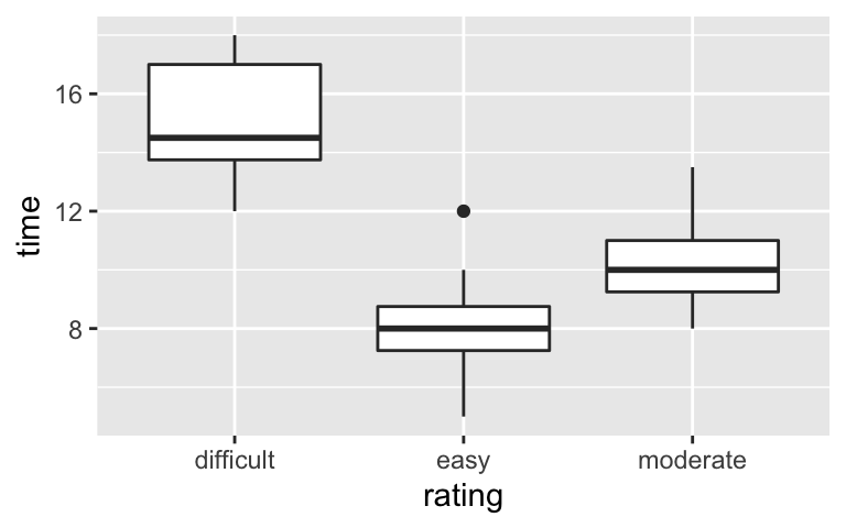
# Model the relationship model_3 <- lm(time ~ rating, data = peaks) confint(model_3) ## 2.5 % 97.5 % ## (Intercept) 13.800649 16.199351 ## ratingeasy -8.576256 -5.423744 ## ratingmoderate -5.921076 -3.190035- How can we interpret the confidence interval for the
ratingmoderatecoefficient? We’re 95% confident that…- the typical completion time of a moderate hike is between 3.19 and 5.92 hours.
- the typical completion time of a moderate hike is between 3.19 and 5.92 hours less than that of a difficult hike.
- the average completion time of moderate hikes in our sample was between 3.19 and 5.92 hours less than that of difficult hikes in our sample.
- the typical completion time of a moderate hike is between 3.19 and 5.92 hours.
- How can we interpret the confidence interval for the intercept coefficient? We’re 95% confident that…
- the typical completion time of a hike with 0 rating is between 13.8 and 16.2 hours.
- the typical completion time of a difficult hike is between 13.8 and 16.2 hours.
- the typical completion time of a difficult hike is between 13.8 and 16.2 hours more than that of an easy hike.
- the typical completion time of a hike with 0 rating is between 13.8 and 16.2 hours.
- How can we interpret the confidence interval for the
18.3 Solutions
Build a sample model
# Take a sample set.seed(34) one_sample_50 <- sample_n(elections, size = 50, replace = FALSE) # Estimate the model one_sample_model <- lm(per_gop_2020 ~ per_gop_2012, one_sample_50) # Check it out coef(summary(one_sample_model)) ## Estimate Std. Error t value Pr(>|t|) ## (Intercept) 11.8822173 3.26519505 3.639053 6.680168e-04 ## per_gop_2012 0.8963895 0.05152905 17.395809 2.309632e-220.8964
0.0515
Pretty close, but a slight underestimate.
- Applying the CLT
- 50%
- 95%
- 5%
- 0.3%
- 50%
- Using the CLT to construct a 95% confidence interval
0.8964 +/- 2*0.0515 = (0.7934, 0.9994)
It was close!
confint(one_sample_model, level = 0.95) ## 2.5 % 97.5 % ## (Intercept) 5.3171027 18.4473320 ## per_gop_2012 0.7927834 0.9999956
- Were we lucky?
No and no!
95% confidence
Roughly 95% of the CIs cover the actual value.set.seed(1) CI_plot(level = 0.95, n = 50)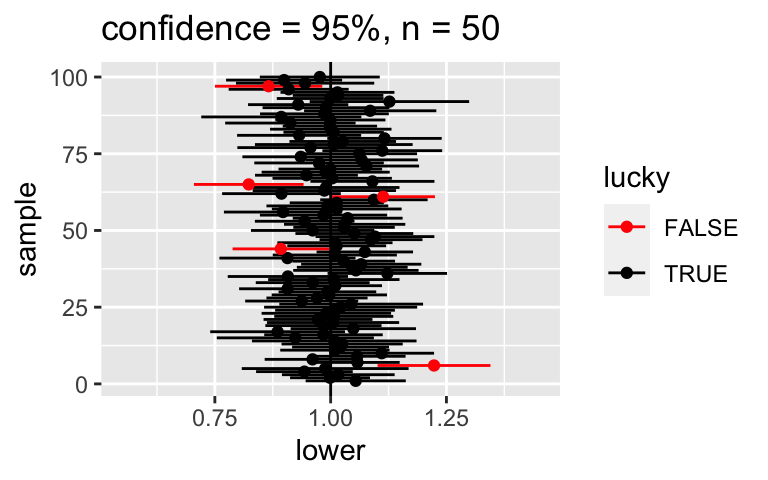
Impact of sample size
will vary
Check your intuition:
set.seed(1)
CI_plot(level = 0.95, n = 200)
95% CIs
Impact of confidence level
Will vary.
\(\hat{\beta}_1\) +/- 1 standard errors
Check your intuition.
# FIRST: For a point of comparison, re-examine the 95% CIs for samples of size 50
CI_plot(level = 0.95, n = 50)
# THEN: Check out 68% CIs for samples of size 50
set.seed(1)
CI_plot(level = 0.68, n = 50)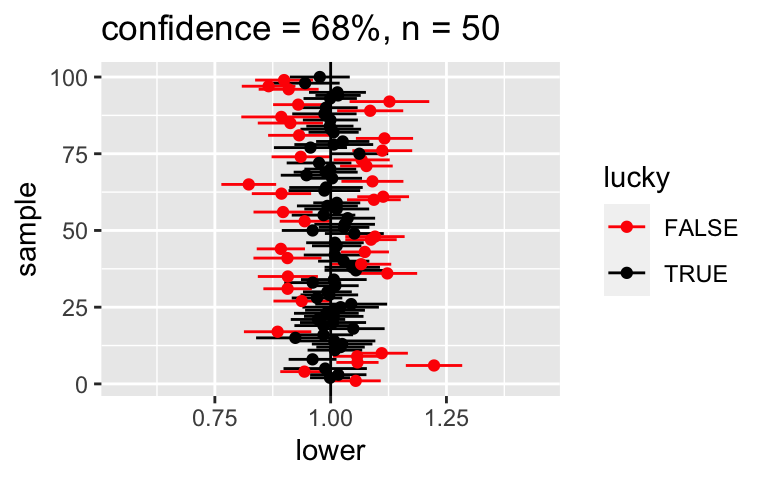
.
set.seed(1)
CI_plot(level = 0.997, n = 50)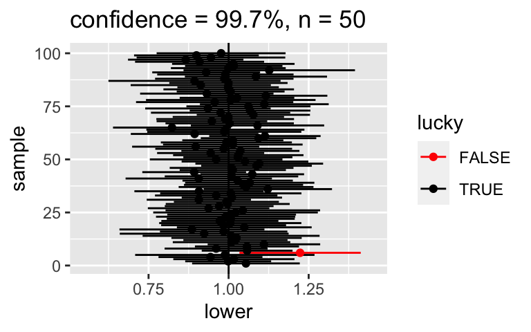
CI_plot(level = 1, n = 50)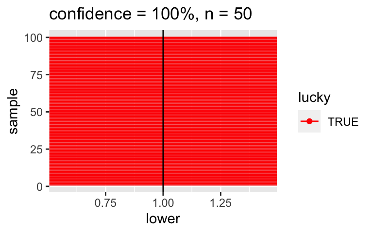
Trade-offs
- increase
- increase
- it provides a too wide or imprecise range of plausible values for the feature we’re trying to estimate
- Traditions
It’s more likely to cover the actual value than an interval with a lower confidence level (eg: 68%) but narrower, hence more useful / precise, than an interval with a higher confidence level (eg: 99.7%).
time versus length – part 1
peaks <- read.csv("https://www.macalester.edu/~ajohns24/data/high_peaks.csv")

# Visualize the relationship
ggplot(peaks, aes(y = time, x = length)) +
  geom_point() +
  geom_smooth(method = "lm", se = FALSE)
# Model the relationship model_1 <- lm(time ~ length, data = peaks) coef(summary(model_1)) ## Estimate Std. Error t value Pr(>|t|) ## (Intercept) 2.0481729 0.80370575 2.548411 1.438759e-02 ## length 0.6842739 0.06161802 11.105095 2.390128e-14will vary
0.684 +/- 2*0.062 = (0.560, 0.808)
.
confint(model_1) ## 2.5 % 97.5 % ## (Intercept) 0.4284104 3.6679354 ## length 0.5600910 0.8084569We’re 95% confident that, for every additional mile in length, completion times increase somewhere between 0.56 and 0.81 hours on average
- time versus length – part 2
Yes! The entire interval is above 0. Thus even when accounting for the potential error in our sample estimate, it seems there’s a positive association between time and length.
time versus elevation
# Visualize the relationship
ggplot(peaks, aes(y = time, x = elevation)) +
  geom_point() +
  geom_smooth(method = "lm", se = FALSE)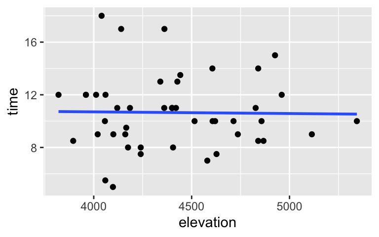
# Model the relationship model_2 <- lm(time ~ elevation, data = peaks) coef(summary(model_2)) ## Estimate Std. Error t value Pr(>|t|) ## (Intercept) 11.2113764116 5.195379956 2.1579512 0.0364302 ## elevation -0.0001269391 0.001175554 -0.1079824 0.9145006will vary
.
confint(model_2) ## 2.5 % 97.5 % ## (Intercept) 0.740776111 21.681976712 ## elevation -0.002496112 0.002242234No! The interval spans negative and positive values, including 0. Thus when accounting for the potential error in our sample estimate, it’s plausible that time is positively associated with elevation, negatively associated with elevation, or not associated at all!
time versus rating
# Visualize the relationship
ggplot(peaks, aes(y = time, x = rating)) +
  geom_boxplot()
# Model the relationship model_3 <- lm(time ~ rating, data = peaks) confint(model_3) ## 2.5 % 97.5 % ## (Intercept) 13.800649 16.199351 ## ratingeasy -8.576256 -5.423744 ## ratingmoderate -5.921076 -3.190035- We’re 95% confident that the typical completion time of a moderate hike is between 3.19 and 5.92 hours less than that of a difficult hike.
- We’re 95% confident that the typical completion time of a difficult hike is between 13.8 and 16.2 hours.