14 Logistic regression: Part II
Announcements
As you get settled in, install the
regclasspackages. Go to the Packages tab in the lower right –> click Install –> type regclass –> click Install. Then test whether this package installed by running this chunk:library(regclass)NOTE: If you get an error, it’s most likely because you are working with an older version of R.
- If you’re working with Mac’s RStudio server, make sure that in the top right of your screen, you see “R 4.1.0”, not “R 4.0.2” or “R 3.6.0”.
- If you’re working with a desktop version of RStudio, you likely didn’t update R at the beginning of this semester. In this case, you have two choices:
- Don’t worry about it. You will be provided with alternative code. It will be more complicated than performing the same task with the
regclasspackage, but it will work. - Download a newer version of R. This does come with the risk of introducing new bugs in the middle of the semester.
- Don’t worry about it. You will be provided with alternative code. It will be more complicated than performing the same task with the
- If you’re working with Mac’s RStudio server, make sure that in the top right of your screen, you see “R 4.1.0”, not “R 4.0.2” or “R 3.6.0”.
Spring break is next week! There won’t be anything due the Tuesday after break.
Homework 5 and Checkpoint 12 will be due the Thursday after break.
14.1 Getting started
Logistic Regression
Let \(y\) be a binary categorical response variable:
\[y =
\begin{cases}
1 & \; \text{ if event happens} \\
0 & \; \text{ if event doesn't happen} \\
\end{cases}\]
Further define
\[\begin{split} p &= \text{ probability event happens} \\ 1-p &= \text{ probability event doesn't happen} \\ \text{odds} & = \text{ odds event happens} = \frac{p}{1-p} \\ \end{split}\]
Then a logistic regression model of \(y\) by \(x\) is \[\log(\text{odds}) = \beta_0 + \beta_1 x\]
We can transform this to get (curved) models of odds and probability:
\[\begin{split} \text{odds} & = e^{\beta_0 + \beta_1 x} \\ p & = \frac{\text{odds}}{\text{odds}+1} = \frac{e^{\beta_0 + \beta_1 x}}{e^{\beta_0 + \beta_1 x}+1} \\ \end{split}\]
Coefficient interpretation for quantitative x
\[\begin{split}
\beta_0 & = \text{ LOG(ODDS) when } x=0 \\
e^{\beta_0} & = \text{ ODDS when } x=0 \\
\beta_1 & = \text{ unit change in LOG(ODDS) per 1 unit increase in } x \\
e^{\beta_1} & = \text{ multiplicative change in ODDS per 1 unit increase in } x \text{ (ie. the odds ratio)} \\
\end{split}\]
Coefficient interpretation for categorical x
\[\begin{split}
\beta_0 & = \text{ LOG(ODDS) at the reference category } \\
e^{\beta_0} & = \text{ ODDS at the reference category } \\
\beta_1 & = \text{ unit change in LOG(ODDS) relative to the reference} \\
e^{\beta_1} & = \text{ multiplicative change in ODDS relative to the reference } \text{ (ie. the odds ratio)} \\
\end{split}\]
Interpreting odds ratios
If \(e^{\beta_1} = 2\):
- the odds double when we increase x by 1
- the odds are twice as big when we increase x by 1
If \(e^{\beta_1} = 0.5\):
- the odds cut in half when we increase x by 1
- the odds are half (50%) as big when we increase x by 1
EXAMPLE 1: Normal or logistic?
For each scenario below, indicate whether Normal or logistic regression would be the appropriate modeling tool.
We want to model whether or not a person believes in climate change (y) based on their age (x).
We want to model whether or not a person believes in climate change (y) based on their location (x).
We want to model a person’s reaction time (y) by how long they slept the night before (x).
We want to model a person’s reaction time (y) by whether or not they took a nap today (x).
EXAMPLE 2
Load the climbers data:
# Load data and packages
library(ggplot2)
library(dplyr)
climbers_sub <- read.csv("https://www.macalester.edu/~ajohns24/data/climbers_sub.csv") %>%
select(peak_name, success, age, oxygen_used, year)- To better understand how climbing success rates have changed over time, let’s model success by year.
#climb_model_1 <- ___(success ~ year, data = climbers_sub, ___)
#coef(summary(climb_model_1))
- Write out the model formula.
___ = -119.36215 + 0.05934year
- Interpret both model coefficients on the odds scale.
exp(-119.36215)
## [1] 1.451032e-52
exp(0.05934)
## [1] 1.061136
EXAMPLE 3
It’s the year 2022. Based on our model, the probability that a climber successfully climbs their peak is roughly 0.65:
# By hand: approach 1 (first calculate odds)
exp(-119.36215 + 0.05934*2022)
## [1] 1.865129
1.865129 / (1 + 1.865129)
## [1] 0.6509756

# By hand: approach 2 (go straight to probability)
exp(-119.36215 + 0.05934*2022)/ (1 + exp(-119.36215 + 0.05934*2022))
## [1] 0.6509755

# Check our work
#predict(climb_model_1, newdata = data.frame(year = 2022), type = "response")- Suppose we had to boil the probability prediction down into a yes / no prediction. Yes or no: do you predict that a climber in 2022 will be successful?
- In logistic regression, we don’t measure the accuracy of a prediction by a residual. Our prediction is either right or wrong. For example, suppose that a given climber this year fails to summit their peak. Was our prediction right or wrong?
14.2 Exercises
climb_model_2:successvsoxygen_used
Next, let’s explore the relationship betweensuccessand the categoricaloxygen_usedpredictor:climb_model_2 <- glm(success ~ oxygen_used, climbers_sub, family = "binomial") coef(summary(climb_model_2)) ## Estimate Std. Error z value Pr(>|z|) ## (Intercept) -1.327993 0.0639834 -20.75528 1.098514e-95 ## oxygen_usedTRUE 2.903864 0.1257404 23.09412 5.304291e-118Check out and summarize a plot of the relationship between success and oxygen use.
# A plot of oxygen_used and success
#ggplot(climbers_sub, aes(x = oxygen_used, fill = ___)) +
#  geom_bar()
Predict the odds and probability of success for a climber that does NOT use oxygen.
# Odds prediction
# exp(-1.327993 + 2.903864*___)

# Probability prediction
Predict the odds and probability of success for a climber that DOES use oxygen.
# Odds prediction
# exp(-1.327993 + 2.903864*___)

# Probability prediction
Calculate and interpret the following odds ratio: divide the odds of success for a climber that does use oxygen by the odds of success for a climber that doesn’t use oxygen. By what degree do the odds increase when oxygen is used?
- Interpretation
How can we interpret the intercept coefficient from
climb_model_2on the odds scale?exp(-1.327993) ## [1] 0.2650086- The odds of success for people that use oxygen are roughly 0.27.
- The odds of success for people that don’t use oxygen are roughly 0.27.
- The odds of success for people that use oxygen are roughly one quarter (27%) as big as the odds of success for people that don’t use oxygen.
On the odds scale, interpret the
oxygen_usedTRUEcoefficient. THINK: Where have you seen this number before?!exp(2.903864) ## [1] 18.24451- The odds of success for people that use oxygen are roughly 18.
- The odds of success for people that don’t use oxygen are roughly 18.
- The odds of success for people that use oxygen are roughly 18 times greater than the odds of success for people that don’t use oxygen.
climb_model_3:successvsageandoxygen_used
Just as with Normal regression, we can utilize more than 1 predictor in a logistic regression model. Let’s try it!climb_model_3 <- glm(success ~ age + oxygen_used, climbers_sub, family = "binomial") coef(summary(climb_model_3)) ## Estimate Std. Error z value Pr(>|z|) ## (Intercept) -0.51957247 0.207331212 -2.506002 1.221049e-02 ## age -0.02197407 0.005459778 -4.024718 5.704361e-05 ## oxygen_usedTRUE 2.89559690 0.126370801 22.913496 3.408591e-116Construct and summarize a plot of this model on the probability scale:
ggplot(___, aes(x = ___, color = ___, y = as.numeric(success))) +
  geom_smooth(method = "glm", method.args = list(family = "binomial"), se = FALSE, fullrange = TRUE) +
  labs(y = "probability of success")

# Just for fun zoom out!
ggplot(___, aes(x = ___, color = ___, y = as.numeric(success))) +
  geom_smooth(method = "glm", method.args = list(family = "binomial"), se = FALSE, fullrange = TRUE) +
  labs(y = "probability of success") +
  lims(x = c(-300, 400))
Interpret the 2 non-intercept coefficients on the odds scale. Don’t forget to “control for…”!
Model evaluation – One climber
We’ve now considered 3 models of climbing success:model predictors climb_model_1year climb_model_2oxygen_used climb_model_3oxygen_used, age If our goal is to obtain accurate predictions of success, which model is best? To this end, let’s consider just the 171st climber in the dataset. This 36-year-old climbed Cho Oyu in 1996, using oxygen, and was not successful:
# Note the new syntax
climbers_sub[171, ]
##     peak_name success age oxygen_used year
## 171   Cho Oyu   FALSE  36        TRUE 1996
Next, use our models to predict the probability of success for this climber:
# Note that we can just plug this climber into newdata
predict(climb_model_1, newdata = climbers_sub[171, ], type = "response")
##       171
## 0.2855754
predict(climb_model_2, newdata = climbers_sub[171, ], type = "response")
##      171
## 0.828619
predict(climb_model_3, newdata = climbers_sub[171, ], type = "response")
##       171
## 0.8299055
Which model(s) correctly predicted that this climber would not succeed, i.e. assigned a probability of success of under 0.5?
Model evaluation – Confusion matrix
It’s not fair to evaluate and compare our models using the performance on just one climber. Instead, we can use a confusion matrix to summarize how the actual outcomes of all climbers compare to the models’ predictions. Construct the confusion matrix forclimb_model_1:# If you have the regclass package: library(regclass) confusion_matrix(climb_model_1) ## Predicted FALSE Predicted TRUE Total ## Actual FALSE 1055 214 1269 ## Actual TRUE 581 226 807 ## Total 1636 440 2076# If you don't have the regclass package: # climbers_sub %>% # select(success) %>% # na.omit() %>% # mutate(predicted = climb_model_1$fitted.values >= 0.5) %>% # count(success, predicted)The confusion matrix contains 3 important metrics. First, show that this model has an overall accuracy rate of 61.7%. That is, it correctly predicted the outcome of 61.7% of all climbers. HINT: Divide the total number of correct predictions by the total number of climbers.
Second, show that this model has a sensitivity, or true positive rate, of only 28.0%. That is, it correctly predicted success for only 28.0% of the successful climbers. HINT: Divide the number of successful climbers that were correctly predicted by the total number of successful climbers.
Finally, show that this model has a specificity, or true negative rate, of only 83.1%. That is, it correctly predicted unsuccessful outcomes for 83.1% of the unsuccessful climbers.
- More confusion matrices
Obtain the confusion matrix, overall accuracy, sensitivity (true positive rate), and specificity (true negative rate) for
climb_model_2. NOTE: The correct metrics are outlined in the next exercise if you want to check your work.# Confusion matrix # Overall accuracy # Sensitivity # SpecificityTake the same steps for
climb_model_3:# Confusion matrix # Overall accuracy # Sensitivity # Specificity
Model comparison
We’ve now considered 3 models of climbing success:model predictors overall sensitivity specificity 1 year 0.617 0.280 0.831 2 oxygen_used 0.802 0.617 0.919 3 oxygen_used, age 0.802 0.617 0.919 - Which model(s) had the highest overall accuracy?
- Which model(s) were the best at predicting when a climber would not succeed, i.e. have the highest specificity?
- In the world of mountain climbing, what do you think is more important: sensitivity (accurately predicting when someone will succeed) or specificity (accurately predicting when someone won’t succeed)?
- Note that the evaluation metrics are the same for
climb_model_2andclimb_model_3. What does this tell you about the age predictor?
- Which of the 3 models is best? (There is a correct answer to this question!)
- Which model(s) had the highest overall accuracy?
14.3 Solutions
climb_model_2:successvsoxygen_usedclimb_model_2 <- glm(success ~ oxygen_used, climbers_sub, family = "binomial") coef(summary(climb_model_2)) ## Estimate Std. Error z value Pr(>|z|) ## (Intercept) -1.327993 0.0639834 -20.75528 1.098514e-95 ## oxygen_usedTRUE 2.903864 0.1257404 23.09412 5.304291e-118.
# A plot of oxygen_used and success
ggplot(climbers_sub, aes(x = oxygen_used, fill = success)) +
  geom_bar()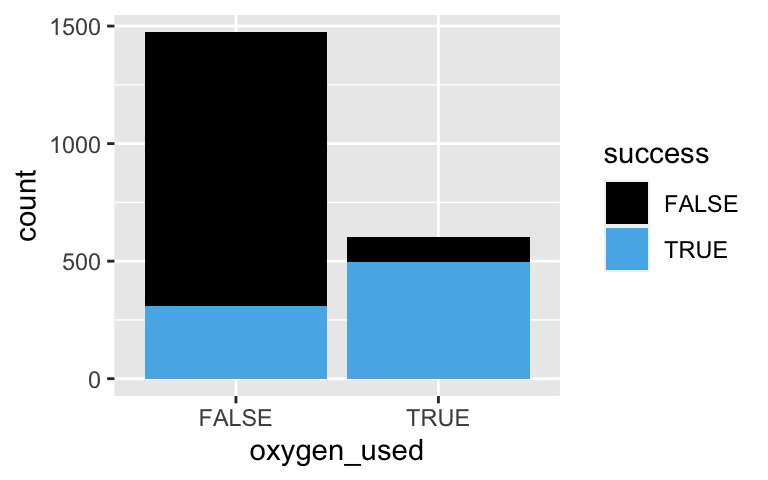
.
# odds
exp(-1.327993 + 2.903864*0)
## [1] 0.2650086

# probability
exp(-1.327993) / (exp(-1.327993) + 1)
## [1] 0.2094915
.
# odds
exp(-1.327993 + 2.903864*1)
## [1] 4.834951

# probability
exp(-1.327993 + 2.903864*1) / (exp(-1.327993 + 2.903864*1) + 1)
## [1] 0.828619
The odds of success are 18 times higher for those that use oxygen.
4.834951 / 0.2650086
## [1] 18.24451
- Interpretation
- The odds of success for people that don’t use oxygen are roughly 0.27.
- The odds of success for people that use oxygen are roughly 18 times greater than the odds of success for people that don’t use oxygen.
- The odds of success for people that don’t use oxygen are roughly 0.27.
climb_model_3:successvsageandoxygen_usedclimb_model_3 <- glm(success ~ age + oxygen_used, climbers_sub, family = "binomial") coef(summary(climb_model_3)) ## Estimate Std. Error z value Pr(>|z|) ## (Intercept) -0.51957247 0.207331212 -2.506002 1.221049e-02 ## age -0.02197407 0.005459778 -4.024718 5.704361e-05 ## oxygen_usedTRUE 2.89559690 0.126370801 22.913496 3.408591e-116.
ggplot(climbers_sub, aes(x = age, color = oxygen_used, y = as.numeric(success))) +
  geom_smooth(method = "glm", method.args = list(family = "binomial"), se = FALSE, fullrange = TRUE) +
  labs(y = "probability of success")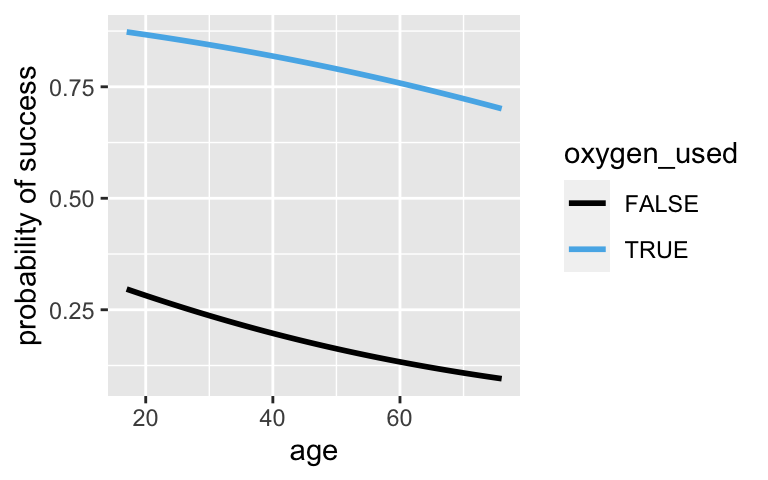
# Just for fun zoom out!
ggplot(climbers_sub, aes(x = age, color = oxygen_used, y = as.numeric(success))) +
  geom_smooth(method = "glm", method.args = list(family = "binomial"), se = FALSE, fullrange = TRUE) +
  labs(y = "probability of success") +
  lims(x = c(-300, 400))
When controlling for oxygen use, the odds of success among people at a given age are 97.8% of what they are among people at the previous age. When controlling for age, the odds of success are roughly 18 times higher when oxygen is useds.
exp(-0.02197407)
## [1] 0.9782656
exp(2.89559690)
## [1] 18.0943
Model evaluation – One climber
Model 1 was correct.# Observed data climbers_sub[171, ] ## peak_name success age oxygen_used year ## 171 Cho Oyu FALSE 36 TRUE 1996 # Predictions predict(climb_model_1, newdata = climbers_sub[171, ], type = "response") ## 171 ## 0.2855754 predict(climb_model_2, newdata = climbers_sub[171, ], type = "response") ## 171 ## 0.828619 predict(climb_model_3, newdata = climbers_sub[171, ], type = "response") ## 171 ## 0.8299055
Model evaluation – Confusion matrix
confusion_matrix(climb_model_1)
##              Predicted FALSE Predicted TRUE Total
## Actual FALSE            1055            214  1269
## Actual TRUE              581            226   807
## Total                   1636            440  2076

# a
(1055 + 226) / 2076
## [1] 0.617052

# b
226 / 807
## [1] 0.2800496

# c
1055 / 1269
## [1] 0.8313633
- More confusion matrices
.
# Confusion matrix
confusion_matrix(climb_model_2)
##              Predicted FALSE Predicted TRUE Total
## Actual FALSE            1166            103  1269
## Actual TRUE              309            498   807
## Total                   1475            601  2076

# Overall accuracy
(1166 + 498) / 2076
## [1] 0.8015414

# Sensitivity
498 / 807
## [1] 0.6171004

# Specificity
1166 / 1269
## [1] 0.9188337
This is the same exact table as for model 2, thus all of the metrics are the same:
# Confusion matrix
confusion_matrix(climb_model_3)
##              Predicted FALSE Predicted TRUE Total
## Actual FALSE            1166            103  1269
## Actual TRUE              309            498   807
## Total                   1475            601  2076
Model comparison
We’ve now considered 3 models of climbing success:model predictors overall sensitivity specificity 1 year 0.617 0.280 0.831 2 oxygen_used 0.802 0.617 0.919 3 oxygen_used, age 0.802 0.617 0.919 - models 2 and 3
- models 2 and 3
- In my opinion, specificity. Climbing can be dangerous and so maybe it’s better to anticipate when you might not succeed.
- It’s most likely multicollinear with oxygen usage. We saw in the previous activity that it’s correlated with success, so we don’t think it’s not useful.
- Model 2. It’s more accurate than model 1 and equally as accurate as, though more simple than, model 3.
- models 2 and 3