7 Model evaluation: Part 2

When you get to class

Open today’s Rmd file linked on the day-to-day schedule. Name and save the file.
Knit the Rmd. Notice that it looks different because I added a theme at the top. This is totally optional but fun! To see other themes, visit here. These are just some options for customizing the appearance of your work.

Announcements

Homework 2 and the next checkpoint are due on Tuesday (in 5 days).
Quiz 1 is in two weeks. Please see details on page 7 of the syllabus. I recommend that you review each activity and homework, trying to answer the questions without first looking at your notes.

7.1 Getting started

WHERE ARE WE?

We’ve been building and, subsequently, evaluating statistical models. To this end, there are 3 important questions to ask:

Is it wrong?
Is it fair?
Is it strong?

EXAMPLE

The high_peaks data includes information on hiking trails in the 46 “high peaks” in the Adirondack mountains of northern New York state.⁴

Our goal will be to understand the variability in the time in hours that it takes to complete each hike. In doing so, we’ll separately consider four possible predictors: a hike’s vertical ascent (feet), highest elevation (feet), length (miles), and difficulty rating (easy / moderate / difficult).

# Load useful packages and data
library(ggplot2)
library(dplyr)
peaks <- read.csv("https://www.macalester.edu/~ajohns24/data/high_peaks.csv")

Construct a separate model of time by each predictor:

# Construct a model of time vs length
model_1 <- lm(time ~ length, data = peaks)

# Construct a model of time vs rating
model_2 <- lm(time ~ rating, data = peaks)

# Construct a model of time vs elevation
model_3 <- lm(time ~ elevation, data = peaks)

# Construct a model of time vs ascent
model_4 <- lm(time ~ ascent, data = peaks)

To counter these numerical summaries, obtain a graphical summary of each relationship. Which relationship appears to be the strongest? Or, which variable seems to be the best predictor of the time required to complete the hike?

# Construct a plot of time alone

# Construct a plot of time vs length

# Construct a plot of time vs elevation

# Construct a plot of time vs ascent

# Construct a plot of time vs rating

Measuring model quality

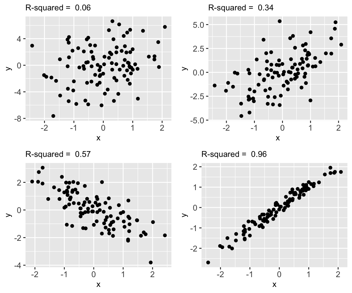
R² provides one rigorous measure of the strength of our model. The following plots illustrate the range of possible R² values:

Interpreting R²

R² measures the proportion of the variability in the observed response values that’s explained by the model. Thus 1 - R² is the proportion of the variability in the observed response values that’s left UNexplained by the model.
$0 \le R^2 \le 1$
The closer R² is to 1, the better the model.

7.2 Exercises

GOALS

Explore R-squared while also reviewing some other modeling concepts.

Warm-up: Data drill
Complete the following tasks using dplyr verbs (filter, summarize, select, mutate, group_by) or using functions like nrow(), head(), etc.

# How many hikes are in the data set?


# Calculate the average elevation


# Calculate the average elevation for each rating


# Define a new variable, length_km, that records the length of a hike in km
# NOTE: 1 mile is roughly 1.6 kilometers


# Calculate the average hiking time


# Calculate the average hiking time for hikes that are more than 14 miles long

Model review: model 1
Re-examine the below plot and model of the relationship between hiking time (in hours) and hike length (in miles). Write down the model formula, interpret the two model coefficients, and use this model to predict the time it takes to complete a 16-mile hike.

# Plot the relationship
ggplot(peaks, aes(y = time, x = length)) + 
  geom_point() + 
  geom_smooth(method = "lm", se = FALSE)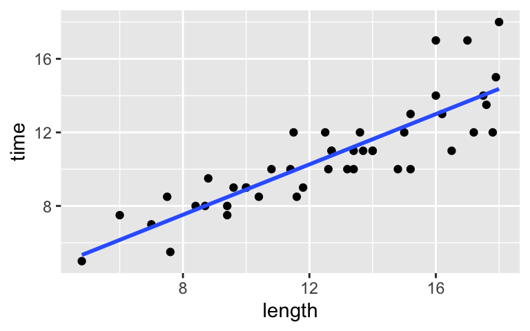


# Summarize the model
summary(model_1)
## 
## Call:
## lm(formula = time ~ length, data = peaks)
## 
## Residuals:
##     Min      1Q  Median      3Q     Max 
## -2.4491 -0.6687 -0.0122  0.5590  4.0034 
## 
## Coefficients:
##             Estimate Std. Error t value Pr(>|t|)    
## (Intercept)  2.04817    0.80371   2.548   0.0144 *  
## length       0.68427    0.06162  11.105 2.39e-14 ***
## ---
## Signif. codes:  0 '***' 0.001 '**' 0.01 '*' 0.05 '.' 0.1 ' ' 1
## 
## Residual standard error: 1.449 on 44 degrees of freedom
## Multiple R-squared:  0.737,  Adjusted R-squared:  0.7311 
## F-statistic: 123.3 on 1 and 44 DF,  p-value: 2.39e-14

Calculating R-squared: model_1
The above scatterplot suggests a relatively strong association between hike time and length. Using R-squared, let’s get a more precise numerical summary of this strength.
1. Upon reviewing summary(model_1) from the previous exercise, confirm that the relationship between time and length has an R-squared value of 0.737. NOTE: Focus on Multiple R-squared and ignore Adjusted R-squared (which we’ll discuss later in the semester).
2. Confirm that we can also obtain R-squared using summary(model_1)$r.squared.
3. Interpret the R-squared value.

Model review: model 2
Re-examine the below plot and model of the relationship between hiking time (in hours) and hike rating. Write down the model formula, interpret the three model coefficients, and use this model to predict the time it takes to complete an easy hike.

# Plot the relationship
ggplot(peaks, aes(y = time, x = rating)) + 
  geom_boxplot()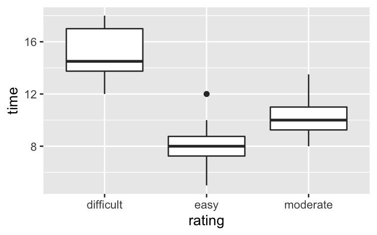


# Summarize the model
summary(model_2)
## 
## Call:
## lm(formula = time ~ rating, data = peaks)
## 
## Residuals:
##     Min      1Q  Median      3Q     Max 
## -3.0000 -1.0000 -0.2222  0.8889  4.0000 
## 
## Coefficients:
##                Estimate Std. Error t value Pr(>|t|)    
## (Intercept)     15.0000     0.5947  25.222  < 2e-16 ***
## ratingeasy      -7.0000     0.7816  -8.956 2.20e-11 ***
## ratingmoderate  -4.5556     0.6771  -6.728 3.19e-08 ***
## ---
## Signif. codes:  0 '***' 0.001 '**' 0.01 '*' 0.05 '.' 0.1 ' ' 1
## 
## Residual standard error: 1.682 on 43 degrees of freedom
## Multiple R-squared:  0.6538, Adjusted R-squared:  0.6377 
## F-statistic:  40.6 on 2 and 43 DF,  p-value: 1.246e-10

Calculating R-squared: model_2
Calculate and interpret the R-squared value for model_2.

Comparing R-squared values
Finally, check out the R-squared values for each model:
```
summary(model_1)$r.squared
## [1] 0.7370358
summary(model_2)$r.squared
## [1] 0.6538002
summary(model_3)$r.squared
## [1] 0.0002649341
summary(model_4)$r.squared
## [1] 0.219844
```
1. Which is the strongest model of hiking time? Similarly, what is the strongest predictor of hiking time?
2. Which is the weakest model? Similarly, what is the weakest predictor of hiking time?

OPTIONAL digging deeper: part 1
Now that we’ve used R-squared, you might wonder how it’s calculated. If so, and especially if you might take more STAT classes, please try these optional exercises. But if you already have enough to chew on, please start working with your group on Homework 2.

To learn about how R-squared is calculated, you’ll use some code that’s specialized to this task. We won’t use it more broadly, so don’t worry about understanding each detail.

Consider model_1 which models time by length. For each hike, we can combine the observed completion time with the model residuals and predictions:
```
# model_1 contains the predictions & residuals for each hike
model_1$fitted.values
model_1$residuals
```
```
# Combine the observed values, predictions, residuals for each hike
model_1_info <- peaks %>% 
  select(time) %>% 
  mutate(predicted = model_1$fitted.values, residual = model_1$residuals)
```
Check out the results. Notice that the observed time values, the predicted time values, and the residuals all vary from hike to hike:
```
head(model_1_info)
```
1. Calculate the variance of the observed time values, predicted values, and residual values for model_3.
2. Repeat this process for model_4, the model of time by ascent. That is, calculate the variances of the observed time values as well as the variances of the predictions and residuals calculated from model_1.

OPTIONAL digging deeper: part 2
Your work for model_1 and model_4 is summarized below, along with additional calculations from model_3.

Model Var(observed) Var(predicted) Var(residuals) R²

model_1 7.810 5.756 2.054 0.74

model_4 7.810 1.717 6.093 0.22

model_3 7.810 0.002 7.808 0.0003
1. No matter the model, the variances of the observed time values are always the same (since we’re using the same raw time values in each model). Further the variances of the observed time values, predictions, and residuals always have the same mathematical relationship. What is it?
2. In general, which models have the most variable predictions and the least variable residuals – the models with higher or lower R-squared?
3. No matter the model, how is R-squared calculated from the variance of the observed values and the variance of their predictions? Congrats! You’ve just established the formula for R².
4. Putting parts c and b together, explain why part b makes sense. That is, why is it desirable for the variability in the predictions to be similar to that in the observed y values? Or, why is it desirable to have small variance in the residuals?

Model	Var(observed)	Var(predicted)	Var(residuals)	R²
`model_1`	7.810	5.756	2.054	0.74
`model_4`	7.810	1.717	6.093	0.22
`model_3`	7.810	0.002	7.808	0.0003

7.3 OPTIONAL – a formula for R-squared

We can partition the variance of the observed response values into the variability that’s explained by the model (the variance of the predictions) and the variability that’s left unexplained by the model (the variance of the residuals):

\[\text{Var(observed) = Var(predicted) + Var(residuals)}\]

“Good” models have residuals that don’t deviate far from 0. So the smaller the variance in the residuals (thus larger the variance in the predictions), the better the model! In pictures:

Putting this together, the R-squared compares Var(predicted) to Var(response):

\[R^2 = \frac{\text{variance of predicted values}}{\text{variance of observed response values}} = 1 - \frac{\text{variance of residuals}}{\text{variance of observed response values}}\]

Finally, IF you like mathematical formulas: Suppose we have a sample of $n$ response values $(y_1,...,y_n)$ that have an average (mean) of $\overline{y}$. Let $\hat{y}_i$ be the prediction of $y_i$ calculated from the model and $y_i - \hat{y}_i$ be the corresponding residual. Then

\[ R^2 = \frac{\sum_{i=1}^n(\hat{y}_i - \overline{y})^2}{\sum_{i=1}^n(y_i - \overline{y})^2} = 1 - \frac{\sum_{i=1}^n(y_i - \hat{y}_i)^2}{\sum_{i=1}^n(y_i - \overline{y})^2} \]

7.4 Solutions

Warm-up: Data drill

# How many hikes are in the data set?
nrow(peaks)
## [1] 46

# Calculate the average elevation
peaks %>% 
  summarize(mean(elevation))
##   mean(elevation)
## 1        4405.283

# Calculate the average elevation for each rating
peaks %>% 
  group_by(rating) %>% 
  summarize(mean(elevation))
## # A tibble: 3 × 2
##   rating    `mean(elevation)`
##   <chr>                 <dbl>
## 1 difficult             4527.
## 2 easy                  4273 
## 3 moderate              4423.


# Define a new variable, length_km, that records the length of a hike in km
# NOTE: 1 mile is roughly 1.6 kilometers
peaks %>% 
  mutate(length_km = length * 1.6) %>% 
  head()
##              peak elevation difficulty ascent length time    rating length_km
## 1     Mt. Marcy        5344          5   3166   14.8 10.0  moderate     23.68
## 2 Algonquin Peak       5114          5   2936    9.6  9.0  moderate     15.36
## 3   Mt. Haystack       4960          7   3570   17.8 12.0 difficult     28.48
## 4   Mt. Skylight       4926          7   4265   17.9 15.0 difficult     28.64
## 5 Whiteface Mtn.       4867          4   2535   10.4  8.5      easy     16.64
## 6       Dix Mtn.       4857          5   2800   13.2 10.0  moderate     21.12


# Calculate the average hiking time
peaks %>% 
  summarize(mean(time))
##   mean(time)
## 1   10.65217

# Calculate the average hiking time for hikes that are more than 14 miles long
peaks %>% 
  filter(length > 14) %>% 
  summarize(mean(time))
##   mean(time)
## 1   13.43333

Model review: model 1
- time = 2.04817 + 0.68427length
- It doesn’t make sense to really interpret the intercept, the expected time to complete a “0-mile hike”.
- For each additional mile, we expect the hike to take 0.68 more hours (~41 more minutes) to complete.
- We expect it to take around 13 hours.
```
2.04817 + 0.68427*16
## [1] 12.99649
```

Calculating R-squared: model_1
```
summary(model_1)$r.squared
## [1] 0.7370358
```
Hike length explains roughly 74% of the variability in completion times from hike to hike.

Model review: model 2
- time = 15 - 7ratingeasy - 4.5556ratingmoderate
- We expect a difficult hike to take around 15 hours to complete.
- We expect an easy hike to take 7 hours less to complete than a difficult hike.
- We expect a moderate hike to take 4.5556 hours less to complete than a difficult hike.
- We expect an easy hike to take 8 hours (15 - 7).

Calculating R-squared: model_2
$R^2 = 40.6$. The difficulty of a hike explains roughly 40.6% of the variability in completion times from hike to hike.

Comparing R-squared values
1. model_1. hike length is the strongest predictor.
2. model_3. hike elevation is the weakest predictor.

OPTIONAL digging deeper: part 1

# Combine the observed values, predictions, residuals for each hike
model_1_info <- peaks %>% 
  select(time) %>% 
  mutate(predicted = model_1$fitted.values, residual = model_1$residuals)

head(model_1_info)
##   time predicted   residual
## 1 10.0 12.175427 -2.1754272
## 2  9.0  8.617203  0.3827973
## 3 12.0 14.228249 -2.2282490
## 4 15.0 14.296676  0.7033236
## 5  8.5  9.164622 -0.6646219
## 6 10.0 11.080589 -1.0805889

# a
model_1_info %>% 
  summarize(var(time), var(predicted), var(residual))
##   var(time) var(predicted) var(residual)
## 1  7.809662          5.756      2.053662

# b
model_4_info <- peaks %>% 
  select(time) %>% 
  mutate(predicted = model_4$fitted.values, residual = model_4$residuals)
model_4_info %>% 
  summarize(var(time), var(predicted), var(residual))
##   var(time) var(predicted) var(residual)
## 1  7.809662       1.716908      6.092754

OPTIONAL digging deeper: part 2
1. var(observed values) = var(predictions) + var(residuals)
2. models with higher R-squared
3. var(predictions) / var(observed values)
4. We want the predictions to be as similar to the observed values as possible, thus we want the variability in the predictions to be similar to that in the observed y values. Similarly, we want the predictions to vary as little from 0 as possible.

original data source = HighPeaks data in the Stat2Data package; original image source = https://commons.wikimedia.org/wiki/File:New_York_state_geographic_map-en.svg ↩︎