4 Balancing & updating
GOALS
Explore, specify, and summarize the balance that a posterior model strikes between our prior and data.
Understand how this balance is updated as more and more data come in.
RECOMMENDED READING
Bayes Rules! Chapter 4.
REVIEW: The Beta-Binomial model
Framework:
- parameter = proportion \(\pi \in [0,1]\)
- data = \(Y\) is the number of successes in \(n\) independendent trials, each with probability of success \(\pi\)
Model:
\[\begin{split} Y|\pi & \sim Bin(n,\pi) \\ \pi & \sim Beta(\alpha,\beta) \\ \end{split} \;\; \Rightarrow \;\; \pi|(Y=y) \sim Beta(\alpha + y, \beta+n-y)\]
Properties:
The Beta is a conjugate prior for \(\pi\) since it produces a Beta posterior. Further:
\[\begin{array}{rlcrl} E(\pi) & = \frac{\alpha}{\alpha + \beta} & \hspace{0.5in} & E(\pi | Y=y) & = \frac{\alpha + y}{\alpha + \beta + n} \\ \text{Mode}(\pi) & = \frac{\alpha - 1}{\alpha + \beta - 2} \;\; \text{ when } && \text{Mode}(\pi | Y=y) & = \frac{\alpha + y - 1}{\alpha + \beta + n - 2} \;\; \text{ when }\\ & \alpha, \beta > 1 && & \alpha + y, \beta + n - y > 1 \\ SD(\pi) & = \sqrt{\frac{\alpha\beta}{(\alpha + \beta)^2(\alpha + \beta+1)}} && SD(\pi | Y=y) & = \sqrt{\frac{(\alpha+y)(\beta+ n-y)}{(\alpha + \beta + n)^2(\alpha + \beta+n+1)}} \\ \end{array}\]
4.1 Warm-up
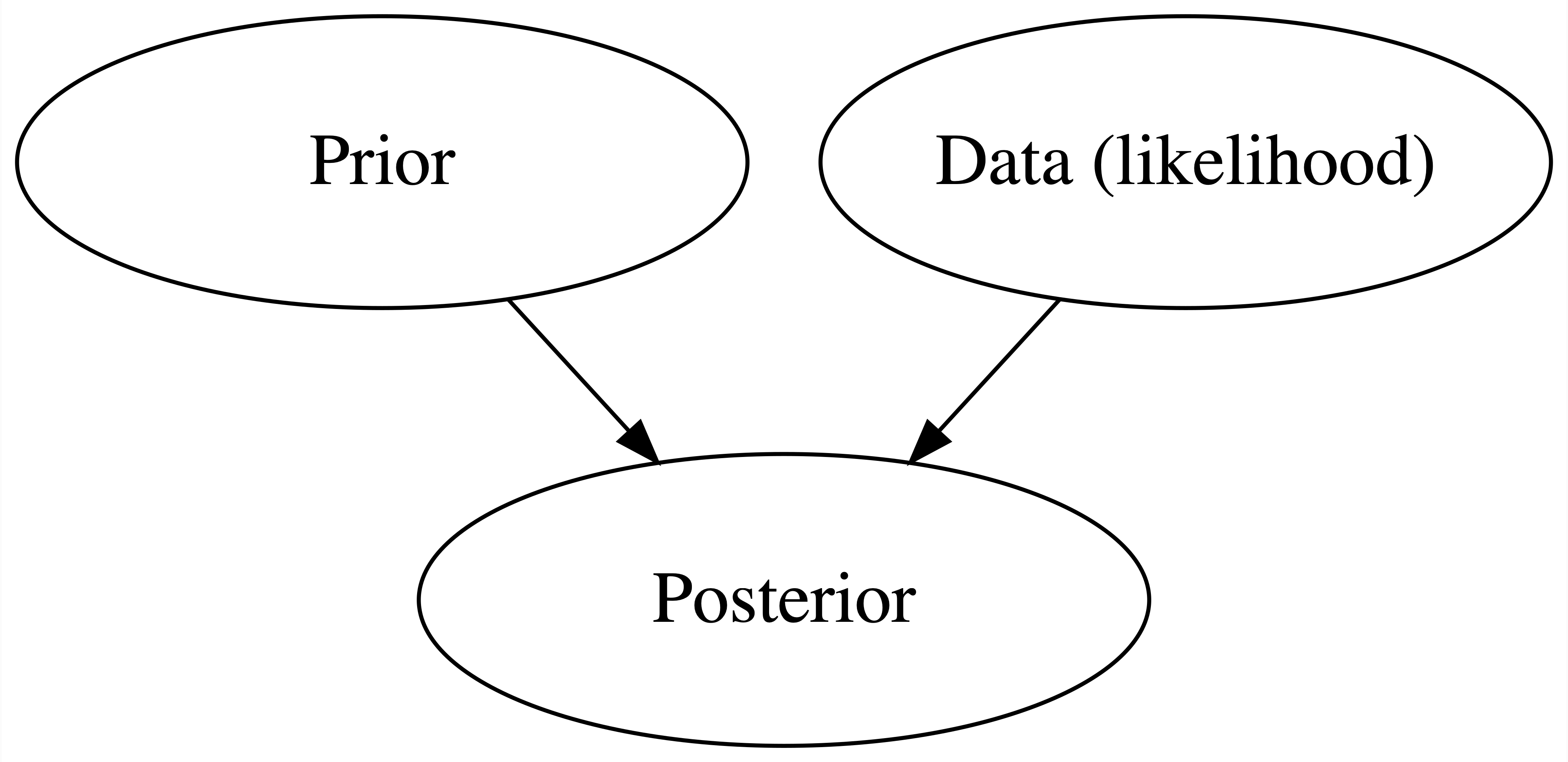
Bayes’ Rule provides the framework for balancing our prior understanding of some parameter \(\pi\) with our observed data \(Y = y\) to construct a posterior understanding of \(\pi\):
EXAMPLE
Let \(\pi \in [0,1]\) be your support in the upcoming MCSG election. As a careful candidate, you interview 3 potential campaign managers.
Each potential manager has their own prior for \(\pi\). Which analyst is the most “sure” about \(\pi\)? Which is the least sure / has the least specific incoming information about \(\pi\)?
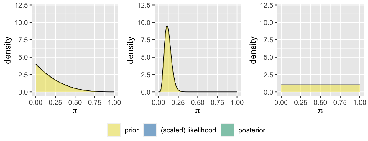
In the first poll, \(Y=6\) of 10 students supported you. Given access to this same data, reflect on what you expect each campaign manager’s posterior to look like. The posterior for Analyst 1 (who you met in Activity 3) is given to you.
Properties of Priors
Priors are tuned to reflect an analyst’s prior understanding about a model parameter. These might be tuned using previous studies, previous data, subject matter knowledge, or theory. The examples above illustrate different types of priors:
informative prior
In general, informative priors have small variance that reflect great a priori certainty. These are typically tuned using expert information (from past studies, etc).vague / uninformative prior
In general, vague priors have large variance that reflect great a priori uncertainty. There are some exceptions – priors with large variance that are actually quite informative on transformed scales.
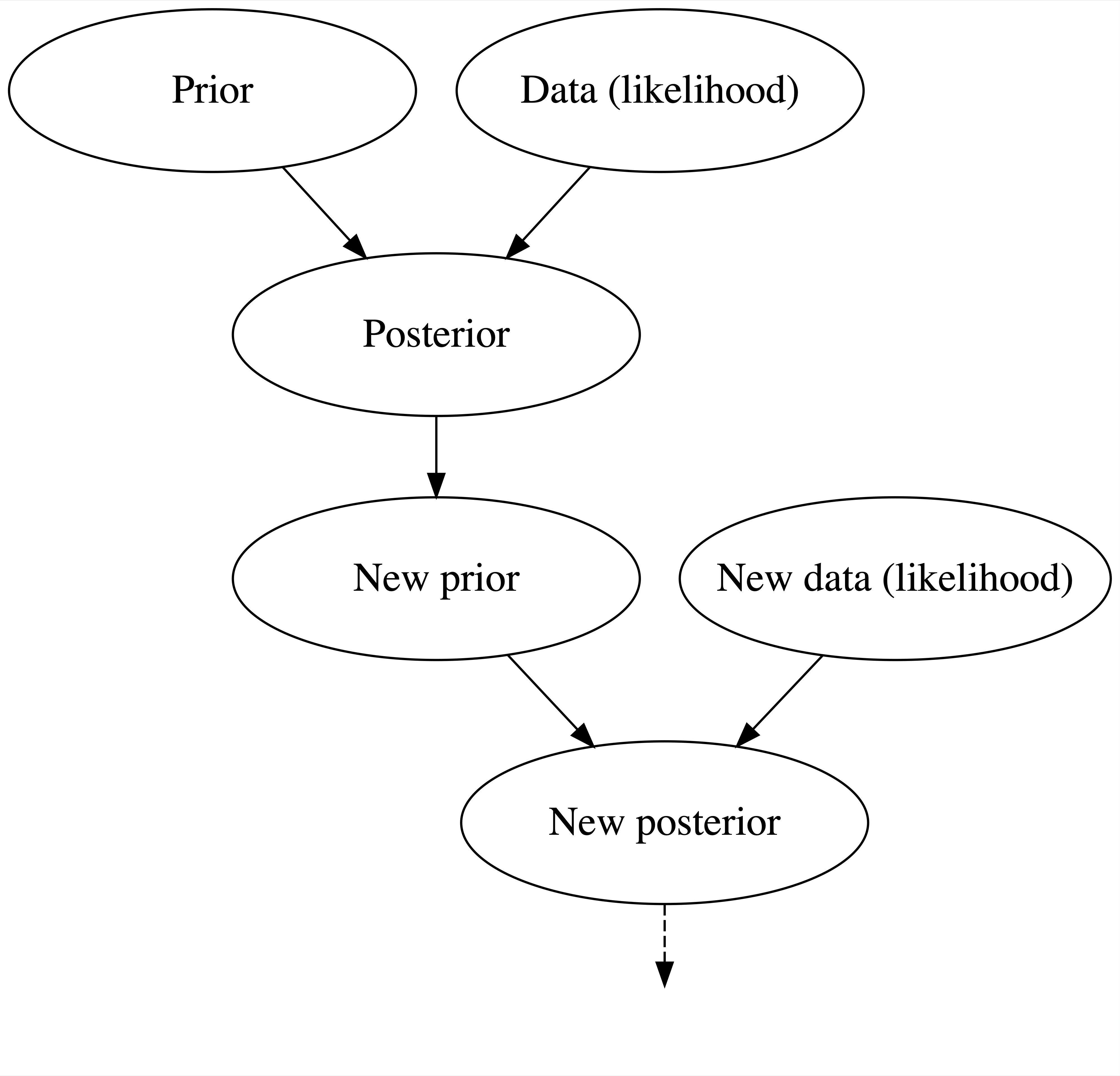
Just as we continually update our understanding of the world as we live life, our posterior balance continues to evolve as new data come in. For example, our understanding of your election support \(\pi\) changes every time we conduct more polls. This is referred to as a SEQUENTIAL BAYESIAN ANALYSIS:
EXAMPLES
How to think like an Epidemiologist outlines the power of sequential Bayesian thinking in the COVID pandemic.
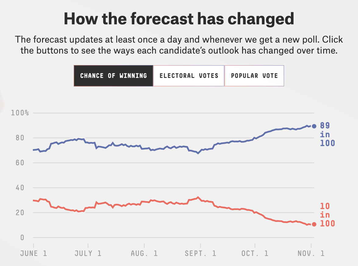
fivethirtyeight.com is famous for using Bayesian models to predict election results. Here’s a snapshot of this evolution across the 2020 campaign season:
Researchers have developed sequential Bayesian methods for use in search-and-rescue efforts (via the SAROPS software). The New York Times highlighted searchers’ use of SAROPS to locate a lost fisherman at sea. A BBC article highlighted the use of similar methods in the search for a missing Malaysia Airlines flight.
Consider some snapshots from a SAROPS presentation. The first image breaks a search area (eg: an ocean region) into a grid. Using ocean drift and weather data, SAROPS assigns each grid square a prior probability for being the location of the missing object - the greater the prior probability, the redder the square. The red lines in the next image depict the searchers’ path. In this scenario they didn’t find the missing object and, in light of this data, updated the grid square probabilities. These probabilities decreased along the already visited search path and increased elsewhere.
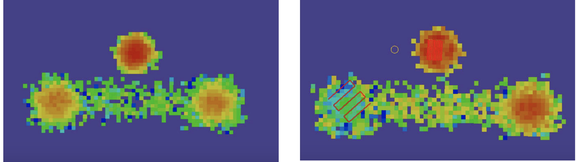
For more details behind this Bayesian search algorithm, you can read this nice stackexchange post.
Does the cover of the course manual make sense now?
4.2 Exercises
4.2.1 Part 1
In Part 1 you’ll explore the posterior understanding of the 3 different analysts that start out with 3 different prior models of your election support \(\pi\). In doing so, the goals will be to explore, specify, and summarize the impact of the prior and data on the posterior.
- Examining the impact of the prior on the posterior
Our 3 analysts observe a poll in which \(Y=6\) of 10 students support you. The prior and resulting posterior models of \(\pi\) are summarized below for the first 2 analysts. Specify the posterior model of \(\pi\) for analyst 3. NOTE: Use the general Beta-Binomial framework, don’t do this from scratch.
analyst prior posterior 1 Beta(1, 4) Beta(7, 8) 2 Beta(7, 50) Beta(13, 54) 3 Beta(1, 1) ??? For each analyst, plot and summarize the Bayesian model using the
plot_beta_binomial()andsummarize_beta_binomial()functions.# Load packages library(bayesrules) # Analyst 1 plot_beta_binomial(alpha = 1, beta = 4, y = 6, n = 10) + ylim(0, 10)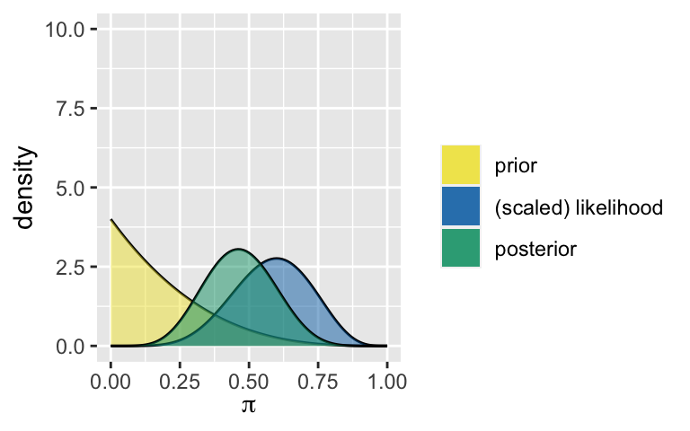
summarize_beta_binomial(alpha = 1, beta = 4, y = 6, n = 10) ## model alpha beta mean mode var sd ## 1 prior 1 4 0.2000000 0.0000000 0.02666667 0.1632993 ## 2 posterior 7 8 0.4666667 0.4615385 0.01555556 0.1247219 # Analyst 2 # Analyst 3Each analyst saw the same data. Yet, they weighed this data against different incoming knowledge and so have different outgoing knowledge. Summarize the punchlines. What’s the point?
No need to worry
It might seem strange that analysts can have different posteriors in light of the same data. In fact, some argue that Bayesian analyses are too subjective – two statisticians can observe the same data and come to different conclusions! In response, consider a quote from John Tukey, a significant figure in the history of statistics (and both a Bayesian & Frequentist):Objectivity is “a fallacy… Economists are not expected to give identical advice in congressional committees. Engineers are not expected to design identical bridges – or aircraft. Why should statisticians be expected to reach identical results from examinations of the same set of data?”
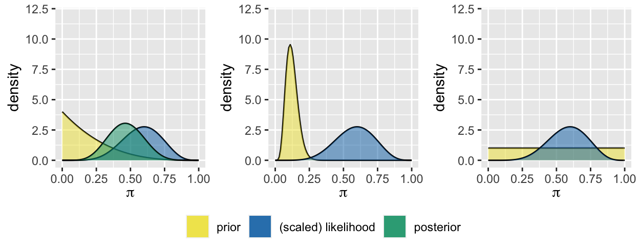
Bolster Tukey’s argument with some reassurance about the potential influence of the prior. Specifically, identify a setting in which the 3 analysts with different priors will have similar posteriors for a poll result in which 60% of people support you. Support your answer with proof from the
plot_beta_binomial()function.
- Reflect and summarize
Bayesian posteriors are a balance between evidence from the prior and data. Reflecting on your above work…- For fixed data, what types of prior models have greater sway over a posterior? Less sway?
- For a fixed prior, when will the data have stronger influence over the posterior – when we have a lot or a little data?
Not only is “subjectivity” not bad, it can be good
The fact that two different priors can lead to different posterior conclusions can actually be a great thing. Let’s revisit an example from the first day of class. Let:- \(\pi_1\) = proportion of Mac students that plan to vote for Trump in 2024
- \(\pi_2\) = proportion of Mac students that can distinguish between coffee and green tea
Tune and specify Beta(\(\alpha, \beta\)) prior models for \(\pi_1\) and \(\pi_2\). Plotting the priors might help:
# pi_1 prior #plot_beta(alpha = ___, beta = ___) # pi_2 prior #plot_beta(alpha = ___, beta = ___)NOTE: Recall that
- Setting \(\alpha = \beta\) gives a prior with \(E(\pi) = 0.5\)
- Setting \(\alpha < \beta\) gives a prior with \(E(\pi) < 0.5\)
- Setting \(\alpha > \beta\) gives a prior with \(E(\pi) > 0.5\)
Suppose that 10 out of 10 students support Trump and 10 out of 10 correctly distinguish between coffee and chai in a taste test. Specify your posterior models of \(\pi_1\) and \(\pi_2\) and visualize them using
plot_beta_binomial():# pi_1 posterior #plot_beta_binomial(alpha = ___, beta = ___, y = 10, n = 10) # pi_2 posterior #plot_beta_binomial(alpha = ___, beta = ___, y = 10, n = 10)
- Reflection
- Did you come to the same posterior conclusions about \(\pi_1\) and \(\pi_2\)?
- How do your posterior conclusions compare with others in the room? How might you come to agreement?
- If you had done a frequentist analysis, what would you conclude about \(\pi_1\) and \(\pi_2\)? How does this compare to your Bayesian conclusions?
4.2.2 Part 2
In Part 1 we explored how the posterior balances the prior and data. In Part 2 we’ll explore the sequential shifts in this balance as more and more data come in. To do so, we’ll continue our election analysis from Analyst 1’s perspective. Recall that they started with a Beta(1,4) prior and, upon observing the first poll in which \(Y = 6\) of 10 voters supported you, ended with a Beta(7, 8) posterior:
plot_beta_binomial(alpha = 1, beta = 4, y = 6, n = 10)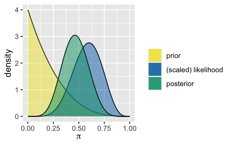
summarize_beta_binomial(alpha = 1, beta = 4, y = 6, n = 10)
## model alpha beta mean mode var sd
## 1 prior 1 4 0.2000000 0.0000000 0.02666667 0.1632993
## 2 posterior 7 8 0.4666667 0.4615385 0.01555556 0.1247219
- A new survey
A new survey has come out! Of 10 students, 3 plan to vote for you. Useplot_beta_binomial()andsummarize_beta_binomial()to plot & summarize the posterior model of \(\pi\). THINK: What’s your prior?!
- Yet another new survey
In the next survey of 20 people, 15 plan to vote for you. Plot & summarize the posterior model of \(\pi\).
Evolution
Your understanding of \(\pi\) evolved as you collected more data: you observed 3 subsequent surveys in which 6 of 10, 3 of 10, and 15 of 20 people planned to vote for you. Confirm that your evolution matches the table below. For reference, also check out the plot of this evolution.survey data model 0 NA Beta(1,4) 1 Y = 6 of n = 10 Beta(7,8) 2 Y = 3 of n = 10 Beta(10,15) 3 Y = 15 of n = 20 Beta(25,20) 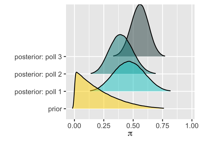
- Another analyst
One of your campaign friends started with the same Beta(1,4), yet learned of the poll results in reverse order: 15 of 20, 3 of 10, and 6 of 10 people planned to vote for you.- Do you think the other analyst’s final conclusions about \(\pi\) are the same as yours?
- Do you think that their evolution in understanding about \(\pi\) looks the same as yours? If not, what do you think it looks like?
- Do you think the other analyst’s final conclusions about \(\pi\) are the same as yours?
Data order invariance
In fact, the new analyst has a different evolution yet ends up with the same posterior model as you. This demonstrates that a sequential Bayesian analysis is invariant to the order in which we observe the data. Confirm that the below summary of their evolution is correct:survey data model 0 NA Beta(1,4) 1 Y = 15 of n = 20 Beta(16,9) 2 Y = 3 of n = 10 Beta(19,16) 3 Y = 6 of n = 10 Beta(25,20) 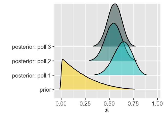
Data dump
There’s a third friend working on your campaign. They start out with the same Beta(1,4) prior for \(\pi\), but unlike the first 2 friends who analyzed the poll results as they received them, the third friend heard about the poll results all at the same time. That is, they heard that of the 40 total students surveyed (10 + 10 + 20), 24 support you (6 + 3 + 15).- What does your gut say: Upon observing these data, what will be the third friend’s posterior?
- Construct the posterior model for this friend. Were you right?
- What does your gut say: Upon observing these data, what will be the third friend’s posterior?
- Challenge: Proving data order invariance & data dumps
The patterns we observed above hold true in any Bayesian analysis. We’ll prove these below. These are also provided in Chapter 4 of Bayes Rules! if you want to check your work.Let’s first prove that Bayesian models are data order invariant. Specifically, start with an original prior pdf \(f(\pi)\). Prove that a sequential analysis in which you observe a first data point \(y_1\) and then a second data point \(y_2\) will produce the same posterior pdf as if you first observed \(y_2\) and then \(y_1\).
Just as the order in which we observe data points doesn’t impact our final posterior, neither does the batching of these data. In general, suppose we observe the collection of two data points \((Y_1,Y_2) = (y_1,y_2)\) where \(Y_1\) and \(Y_2\) are conditionally independent:
\[f(y_1,y_2|\pi) = f(y_1|\pi)f(y_2|\pi)\]
and independent
\[f(y_1,y_2) = f(y_1)f(y_2)\]
Prove that the posterior pdf of \(\pi\) in light of this data collection is the same as the posteriors derived via the sequential analysis in part a.
4.3 Solutions
- Examining the impact of the prior on the posterior
.
analyst prior posterior 1 Beta(1, 4) Beta(7, 8) 2 Beta(7, 50) Beta(13, 54) 3 Beta(1, 1) Beta(7, 5) .
# Load packages
library(bayesrules)

# Analyst 1
plot_beta_binomial(alpha = 1, beta = 4, y = 6, n = 10) +
  ylim(0, 10)
summarize_beta_binomial(alpha = 1, beta = 4, y = 6, n = 10) ## model alpha beta mean mode var sd ## 1 prior 1 4 0.2000000 0.0000000 0.02666667 0.1632993 ## 2 posterior 7 8 0.4666667 0.4615385 0.01555556 0.1247219 # Analyst 2 plot_beta_binomial(alpha = 7, beta = 50, y = 6, n = 10) + ylim(0, 10)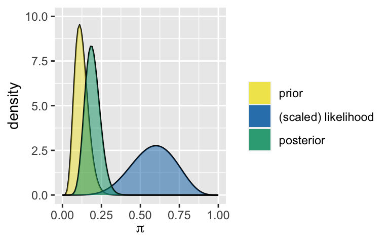
summarize_beta_binomial(alpha = 7, beta = 50, y = 6, n = 10)
##       model alpha beta      mean      mode         var         sd
## 1     prior     7   50 0.1228070 0.1090909 0.001857335 0.04309681
## 2 posterior    13   54 0.1940299 0.1846154 0.002299739 0.04795560

# Analyst 3
plot_beta_binomial(alpha = 1, beta = 1, y = 6, n = 10) +
  ylim(0, 10)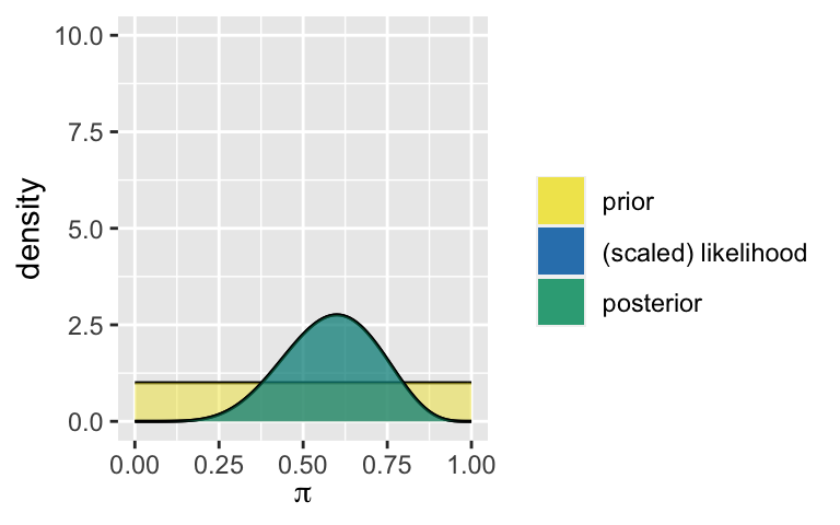
summarize_beta_binomial(alpha = 1, beta = 1, y = 6, n = 10)
##       model alpha beta      mean mode        var        sd
## 1     prior     1    1 0.5000000  NaN 0.08333333 0.2886751
## 2 posterior     7    5 0.5833333  0.6 0.01869658 0.1367354
Think: Who was the most swayed by the data? Why were they the most swayed? Who was the least swayed, ie. the most stubborn? Why were they the least swayed?
No need to worry
Increase sample size. For example, if 600 of 1000 polled students supported you, the posteriors would be similar.plot_beta_binomial(alpha = 1, beta = 4, y = 600, n = 1000) plot_beta_binomial(alpha = 7, beta = 50, y = 600, n = 1000) plot_beta_binomial(alpha = 1, beta = 1, y = 600, n = 1000)g1 <- plot_beta_binomial(alpha = 1, beta = 4, y = 600, n = 1000) g2 <- plot_beta_binomial(alpha = 7, beta = 50, y = 600, n = 1000) g3 <- plot_beta_binomial(alpha = 1, beta = 1, y = 600, n = 1000) grid.arrange(g1,g2,g3,ncol=3)
- Reflect and summarize
- informative. vague.
- a lot
- Not only is “subjectivity” not bad, it can be good
Will vary by student.
- Reflection
Will vary by student.
A new survey Starting at a Beta(7,8) prior, we get a Beta(10,15) posterior.
plot_beta_binomial(7, 8, 3, 10)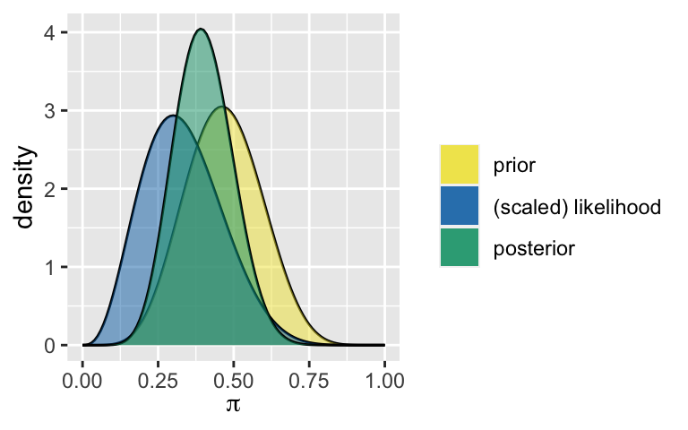
summarize_beta_binomial(7, 8, 3, 10)
##       model alpha beta      mean      mode         var         sd
## 1     prior     7    8 0.4666667 0.4615385 0.015555556 0.12472191
## 2 posterior    10   15 0.4000000 0.3913043 0.009230769 0.09607689
Yet another new survey
Starting at a Beta(10,15) prior, we get a Beta(25,20) posterior.plot_beta_binomial(10, 15, 15, 20)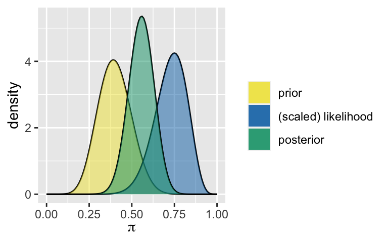
summarize_beta_binomial(10, 15, 15, 20)
##       model alpha beta      mean      mode         var         sd
## 1     prior    10   15 0.4000000 0.3913043 0.009230769 0.09607689
## 2 posterior    25   20 0.5555556 0.5581395 0.005367687 0.07326450
- Evolution
yes it matches up
- Another analyst
Will vary by student.
Data order invariance
In fact, the new analyst has a different evolution yet ends up with the same posterior model as you. This demonstrates that a sequential Bayesian analysis is invariant to the order in which we observe the data. Confirm that the below summary of their evolution is correct:survey data model 0 NA Beta(1,4) 1 Y = 15 of n = 20 Beta(16,9) 2 Y = 3 of n = 10 Beta(19,16) 3 Y = 6 of n = 10 Beta(25,20) # poll 1: starting from a Beta(1,4) prior summarize_beta_binomial(1, 4, 15, 20) ## model alpha beta mean mode var sd ## 1 prior 1 4 0.20 0.0000000 0.026666667 0.16329932 ## 2 posterior 16 9 0.64 0.6521739 0.008861538 0.09413574 # poll 2: starting from a Beta(16,9) prior summarize_beta_binomial(16, 9, 3, 10) ## model alpha beta mean mode var sd ## 1 prior 16 9 0.6400000 0.6521739 0.008861538 0.09413574 ## 2 posterior 19 16 0.5428571 0.5454545 0.006893424 0.08302665 # poll 3: starting from a Beta(19,16) prior summarize_beta_binomial(19, 16, 6, 10) ## model alpha beta mean mode var sd ## 1 prior 19 16 0.5428571 0.5454545 0.006893424 0.08302665 ## 2 posterior 25 20 0.5555556 0.5581395 0.005367687 0.07326450
- Data dump
Will vary.
They end up with the same Beta(25,20) posterior
summarize_beta_binomial(1, 4, 24, 40)
##       model alpha beta      mean      mode         var        sd
## 1     prior     1    4 0.2000000 0.0000000 0.026666667 0.1632993
## 2 posterior    25   20 0.5555556 0.5581395 0.005367687 0.0732645
- Challenge: Proving data order invariance & data dumps
See Chapter 4 of Bayes Rules!.