9 Regression review

GOALS

Thus far, we’ve been building models of one data variable: \(Y\). However, we typically want to understand the relationship between \(Y\) and a set of predictors \((X_1, X_2, \ldots, X_p)\). For example, we might wish to understand how a person’s belief in climate change (\(Y\)) relates to their age (\(X_1\)) and years of education (\(X_2\)). Before taking a Bayesian approach, let’s review some frequentist regression concepts from STAT 155.

BACKGROUND

Let \(Y\) be a response variable and \(X = (X_1,X_2,\ldots,X_p)\) be a set of predictors. Then the Normal regression model of \(Y\) vs \(X\) has

\[Y = \beta_0 + \beta_1X_1 + \cdots + \beta_pX_p + \varepsilon\]

where

\(E(Y|X) = \beta_0 + \beta_1X_1 + \cdots + \beta_pX_p\) is the expected or typical \(Y\) outcome at the given set of predictor values
\(\varepsilon\) = residual error, i.e. how much the observed outcome of \(Y\) deviates from the expected outcome. We assume that these errors are Normally distributed around 0 with some standard deviation \(\sigma\).

To review these concepts, we’ll use data on Capital Bikeshare (a bikeshare service in Washington, D.C.) to model \(Y\), the number of daily rides on any given day, vs a variety of potential predictors \(X\) (e.g. the temperature, day of the week, windspeed, humidity). Each of the 500 rows in this dataset include information about a single day.

# Load packages and data
library(tidyverse)
library(bayesrules)
data("bikes")
bikes %>% 
    dim()
## [1] 500  13

To begin, consider the model of rides (\(Y\)) vs temp_feel (\(X\)) where temp_feel is what the temperature feels like in degrees Fahrenheit when accounting for humidity, etc.

        ggplot(bikes, aes(x = temp_feel, y = rides)) + 
            geom_point() + 
            geom_smooth(method = "lm")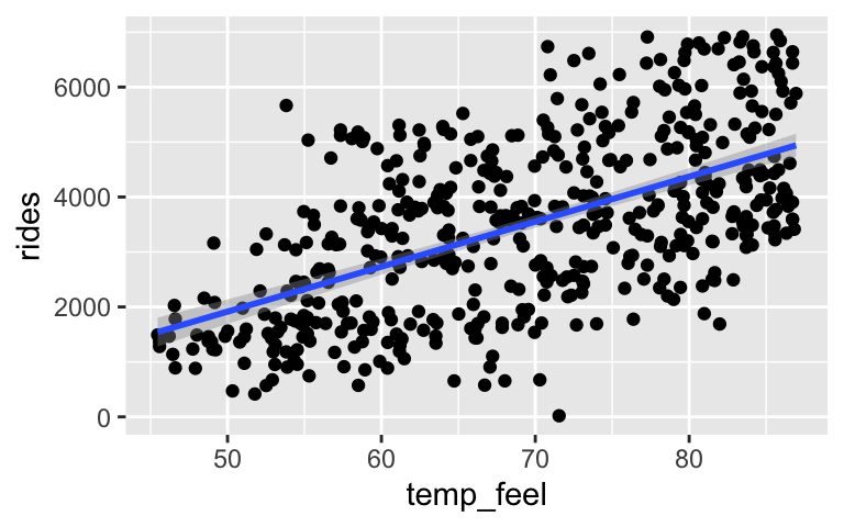

        model_1 <- lm(rides ~ temp_feel, data = bikes)
        coef(summary(model_1))
##                Estimate Std. Error   t value     Pr(>|t|)
## (Intercept) -2179.26863 358.629796 -6.076652 2.441219e-09
## temp_feel      81.87994   5.120101 15.991861 9.292611e-47

 The estimated model equation is `rides = -2179.3 + 81.9 temp_feel`. How can we interpret 81.9?

For every 1 degree increase in temperature, we expect around 81.9 more riders.
For every extra rider, we expect temperature to increase by around 81.9 degrees.
We expect around 81.9 riders on 0-degree days.

Since 0-degree days are far outside the norm for our dataset, we can’t meaningfully interpret the intercept -2179.3. (We can’t say that there are typically -2179.3 rides when temp_feel is 0.) Instead, we can consider the centered intercept, i.e. the typical ridership on days with the typical temperature. Use the model equation above with a mean temperature of 69.1437 to calculate this centered intercept. Round your answer to the nearest whole number.
```
bikes %>% 
    summarize(mean(temp_feel))
##   mean(temp_feel)
## 1         69.1437
```

Next, consider the model of rides by temp_feel:

        ggplot(bikes, aes(x = weekend, y = rides)) + 
            geom_boxplot()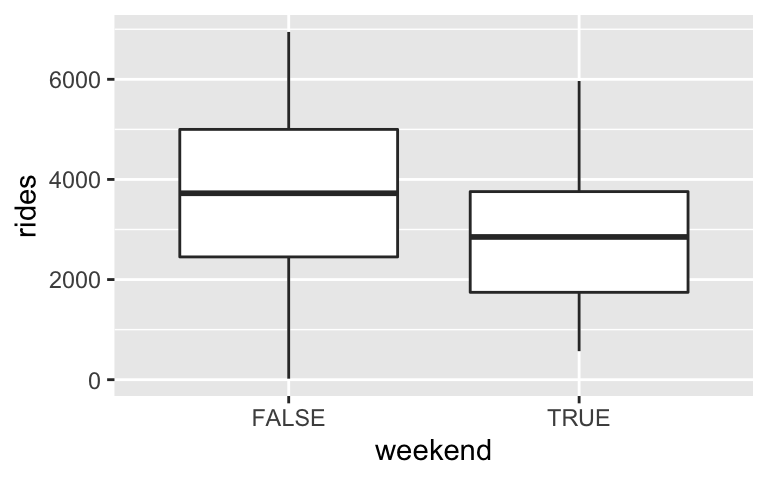

        model_2 <- lm(rides ~ weekend, data = bikes)
        coef(summary(model_2))
##              Estimate Std. Error   t value      Pr(>|t|)
## (Intercept) 3712.1170   80.89871 45.885984 5.423684e-181
## weekendTRUE -815.2588  152.34109 -5.351536  1.332864e-07

 The estimated model equation is `rides = 3712.1 - 815.3 weekendTRUE` where `weekendTRUE` is an *indicator* of weekends -- it's 1 for weekends and 0 otherwise. How can we interpret 3712.1?

We expect 3712 more riders on weekdays than weekends.
We expect 3712 more riders on weekends than weekdays.
We expect 3712 riders on weekends
We expect 3712 riders on weekdays.

How can we interpret -815.3?
1. For each additional weekend, we expect 815 fewer riders.
2. We expect 815 fewer riders on weekdays than weekends.
3. We expect 815 fewer riders on weekends than weekdays.
4. We expect -815 riders on weekends.
5. We expect -815 riders on weekdays.

Predict the number of riders there will be on Saturday. Round your answer to the nearest whole number.

Next, consider the model of rides by both temp_feel and weekend:

        ggplot(bikes, aes(x = temp_feel, y = rides, color = weekend)) + 
            geom_point() +
            geom_smooth(method = "lm")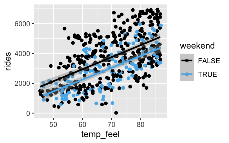

        model_3 <- lm(rides ~ temp_feel + weekend, data = bikes)
        coef(summary(model_3))
##                Estimate Std. Error   t value     Pr(>|t|)
## (Intercept) -1873.75079 351.789563 -5.326340 1.521287e-07
## temp_feel      80.34736   4.971498 16.161601 1.592144e-47
## weekendTRUE  -707.62118 123.643576 -5.723073 1.810601e-08

 The estimated model equation is `rides = -1873.8 + 80.3 temp_feel - 707.6 weekendTRUE`. How can we interpret 80.3?

For every 1 degree increase in temperature, we expect around 80 more riders.
When controlling for day of the week, i.e. on both weekends and weekdays, we expect around 80 more riders for every 1 degree increase in temperature.

How can we interpret -707.6?
1. We expect roughly 708 fewer riders on weekdays than weekends.
2. When controlling for temperature, i.e. at any given temperature, we expect roughly 708 fewer riders on weekends than weekdays.
3. For each additional weekend, we expect 708 fewer riders.
4. When controlling for temperature, i.e. at any given temperature, we expect 708 fewer riders on each additional weekend.

Consider a final model. Interpret the windspeed coefficient, -32.8.

model_4 <- lm(rides ~ temp_feel + weekend + windspeed, data = bikes)
coef(summary(model_4))
##                Estimate Std. Error   t value     Pr(>|t|)
## (Intercept) -1280.10650 393.185742 -3.255730 1.208336e-03
## temp_feel      77.96591   4.978016 15.662044 3.261216e-45
## weekendTRUE  -713.57504 122.477855 -5.826156 1.021390e-08
## windspeed     -32.82144  10.072250 -3.258600 1.196434e-03

Finally, consider a model of \(Y\), the 3pm temperature in Perth, Australia by \(X\), where \(X\) is either 9am temperature or 9am humidity level:

\[Y = \beta_0 + \beta_1 X + \varepsilon\]

Recall our assumption that the residuals \(\varepsilon\) are Normally distributed around 0 with standard deviation \(\sigma\). Based on the scatterplots below, which model has the smaller \(\sigma\): the model of \(Y\) by 9am temperature or the model of \(Y\) by 9am humidity?
```
data("weather_perth")
ggplot(weather_perth, aes(x = temp9am, y = temp3pm)) + 
    geom_point()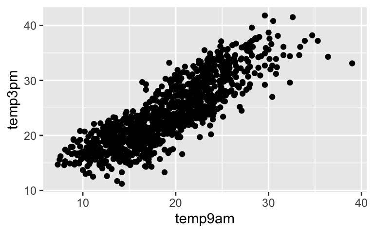
```
```
ggplot(weather_perth, aes(x = humidity9am, y = temp3pm)) + 
    geom_point()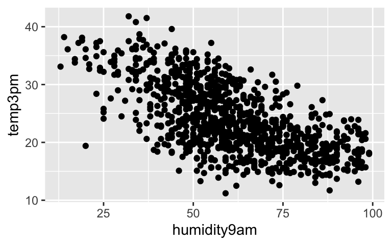
```

If you finish early
Next week we’ll explore Bayesian regression. For example, we could simulate the Bayesian regression model of rides by temp_feel:
```
# Simulate a posterior regression model
# Use default vague priors
bike_model <- stan_glm(
    rides ~ temp_feel, data = bikes,
    family = gaussian,
    chains = 4, iter = 5000*2, seed = 84735)
```
Play around with this model using the MCMC tools you’ve learned thus far.
1. Check out some diagnostics.
2. Report summaries of the model parameters \(\beta_0\), \(\beta_1\), and \(\sigma\). How do these compare with the frequentist summaries?
3. Do we have ample evidence of a positive association between ridership and temperature?
4. How would you write out the structure of this Bayesian model? For example, what’s the “data model?” What priors might be appropriate?