Probability Review

Sample Spaces & Events

VIDEO: Watch this video for a quick tutorial of the concepts below.

Throughout, let $A, B$ be events in sample space $S$, i.e. $A \subseteq S, B \subseteq S$. The following are some “special” events:

$\emptyset$ = the empty / null set containing no outcomes
$A^c$ = “$A$ complement” = all outcomes in $S$ that are not in $A$
$A \cap B$ = “intersection of $A$ and $B$” = all outcomes in both $A$ and $B$
$A$ and $B$ are mutually exclusive or disjoint if $A \cap B = \emptyset$
$A \cup B$ = “union of $A$ and $B$” = all outcomes in $A$ or $B$ or both

Probability, Conditional Probability & Independence

VIDEO: Watch this video for a quick tutorial of the probability concepts below.

Recall the axioms & rules of probability.

Probability

Let $A, B$ be events in sample space $S$. A probability function $P$ must satisfy the following axioms:

$P(\emptyset) = 0$
$P(S) = 1$
If $A \cap B = \emptyset$, then $P(A \cup B) = P(A) + P(B)$.

The following properties follow from these axioms:

$P(A^c) = 1 - P(A)$
If $A \subseteq B$, then $P(A) \le P(B)$
$P(A \cup B) = P(A) + P(B) - P(A \cap B)$

Sometimes we know that a certain event, say $B$, has occurred. This might or might not change the plausibility of another event $A$. The concepts of conditional probability and independence are summarized here.

Conditional Probability

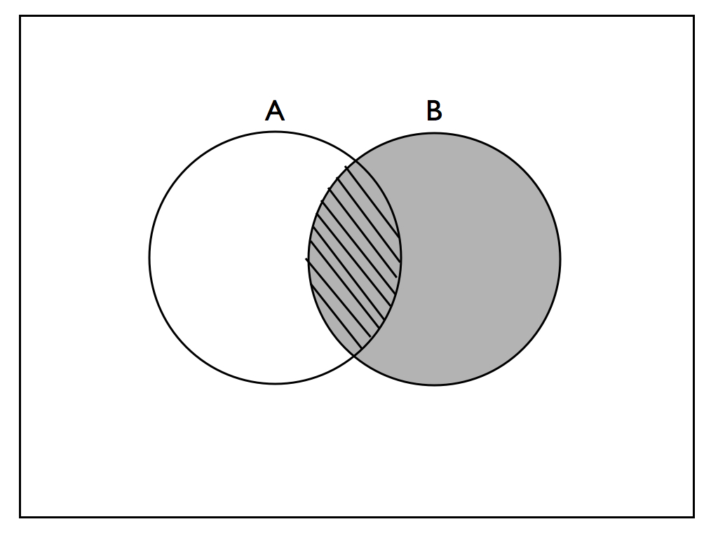
The conditional probability of $A$ given $B$, $P(A | B)$, is the probability of observing $A$ given the knowledge that we’ve observed $B$. In calculating $P(A | B)$, we calculate the likelihood of $A$ relative to the shrunken sample space of $B$:

\[P(A|B) = \frac{P(A\cap B)}{P(B)}\]

This concept is captured in the following image.

Independence

Events $A$ and $B$ are independent if the occurrence of $B$ doesn’t change our information about $A$, i.e. \[P(A|B) = P(A)\] Equivalently, $A$ and $B$ are independent if \[P(A \cap B) = P(A)P(B)\]

In general, let $A_1, A_2, ..., A_k$ be $k$ pairwise independent events. That is, all pairs $A_i$ and $A_j$ for $i \ne j$ and $i,j \in \{1,...,k\}$ are independent. Then \[P\left( \cap_{i=1}^k A_i \right) := P(A_1 \cap A_2 \cap \cdots A_k) = P(A_1)P(A_2)\cdots P(A_k) := \prod_{i=1}^k P(A_i) \; .\]

Random Variables

Let $X, Y$ be random variables (RVs), i.e. numerical functions of a sample space. There are 2 types of RVs:

discrete
Example: $X$ = number of heads in 10 coin flips. Then $X \in \{1,2,...,10\}$.
continuous
Example: $X$ = speed of a car. Then $X \in [0,\infty)$.

Marginal, Joint, & Conditional pdfs

The marginal model of $X$, i.e. the behavior of $X$ ignoring all other variables, is captured by its probability density function (pdf) \[f(x)\] where $f(x)$ describes the possible values of $X$ and their relative likelihoods.

Properties of a marginal pdf

$X$ discrete:

$f(x) = P(\{X=x\})$
$0 \le f(x) \le 1$
$\sum_{\text{all } x} f(x) = 1$

$X$ continuous:

$f(x) \ge 0$ (not a probability)
$\int_{-\infty}^\infty f(x) dx = 1$

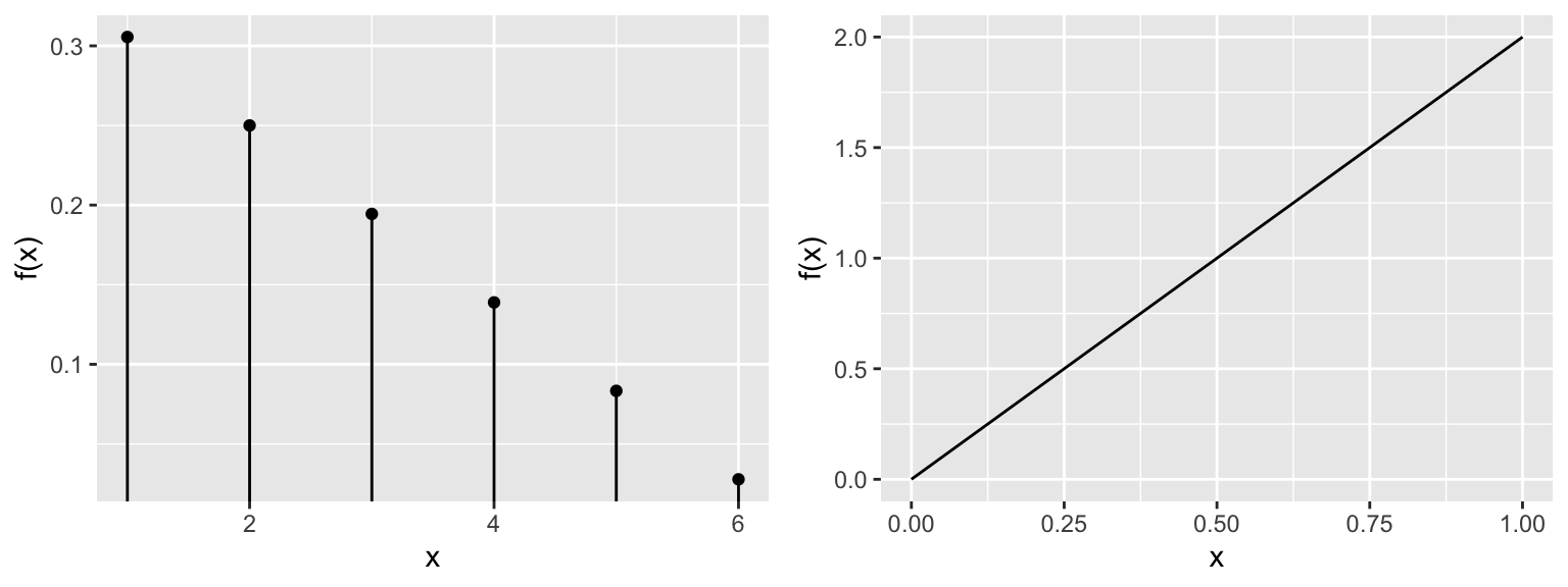
For example, consider a discrete marginal pdf (left) and continuous marginal pdf (right):

The simultaneous behavior of $X$ and $Y$ is described by their joint pdf \[f(x,y)\] where $f(x,y)$ satisfies the following properties.

Properties of a joint pdf

$X, Y$ discrete:

$f(x,y) = P(\{X=x\} \cap \{Y=y\}) = P(X=x, Y=y) \;\; \text{(shorthand)}$
$0 \le f(x,y) \le 1$
$\sum_{\text{all } x} \sum_{\text{all } y} f(x,y) = 1$

$X, Y$ continuous:

$f(x,y) \ge 0$ (not a probability)
$\int_{-\infty}^\infty \int_{-\infty}^\infty f(x,y) dx dy = 1$

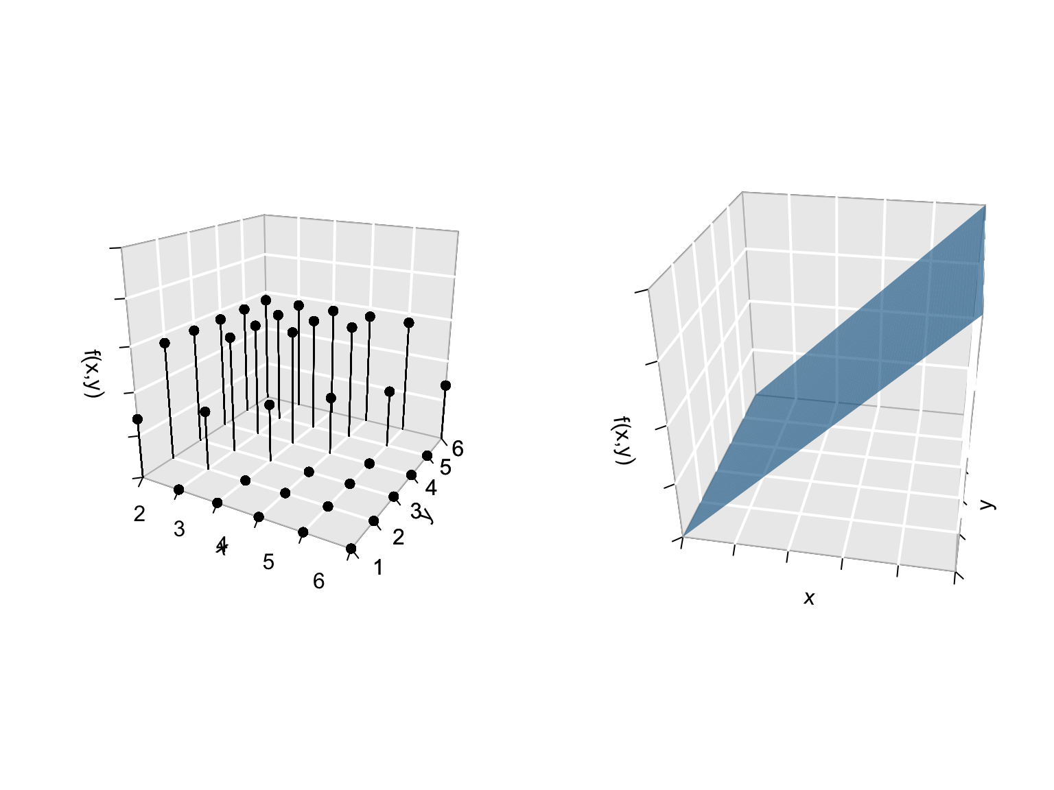
For example, consider a discrete joint pdf (left) and continuous joint pdf (right):

Of course, we can use information about the joint behavior of $X$ and $Y$ to learn about their marginal behaviors.

Connections between the joint and marginal pdfs

$X, Y$ discrete: \[\begin{split} f(x) & = \sum_{all \; y} f(x,y) \\ f(y) & = \sum_{all \; x} f(x,y) \\ \end{split}\]

$X, Y$ continuous: \[\begin{split} f(x) & = \int_{-\infty}^\infty f(x,y) dy \\ f(y) & = \int_{-\infty}^\infty f(x,y) dx \\ \end{split}\]

In some cases, we know the value of $Y$ but not the value of $X$. We can utilize this information if we know the conditional behavior of $X$ when $Y=y$: \[f(x|y)\]

Properties of a conditional pdf

$X,Y$ discrete:

$f(x|y) = P(\{X=x\} | \{Y=y\})$
$0 \le f(x|y) \le 1$
$\sum_{\text{all } x} f(x|y) = 1$

$X,Y$ continuous:

$f(x|y) \ge 0$ (not a probability)
$\int_{-\infty}^\infty f(x|y) dx = 1$

Recall that we can use the marginal probability ($P(B)$) and joint probability ($P(A \cap B)$) to calculate the conditional probability ($P(A|B)$): \[P(A|B) = \frac{P(A \cap B)}{P(B)}\] Similarly, we can calculate the conditional pdf from the marginal and joint pdfs:

Bayes’ Rule & Law of Total Probability extended to pdfs

Bayes’ Rule can be extended to RVs:

\[f(x|y) = \frac{f(x,y)}{f(y)} = \frac{f(y|x)f(x)}{f(y)}\]

where, by the Law of Total probability

\[f(y) = \begin{cases} \sum_{\text{all } x} f(y|x)f(x) & X \text{ discrete} \\ \int f(y|x)f(x)dx & X \text{ continuous} \\ \end{cases}\]

Further, recall that for events $A$ and $B$, we say that $A$ and $B$ are independent if the knowledge of $B$ doesn’t change the plausibility of $A$: \[A,B \text{ independent } \Rightarrow \begin{split} P(A|B) & = P(A) \\ P(A \cap B) & = P(A)P(B) \end{split}\] We can similarly define the independence of 2 random variables.

Independent RVs

RVs $X$ and $Y$ are independent if and only if \[\begin{split} f(x|y) & = f(x) \\ f(x,y) & = f(x)f(y) \\ \end{split}\]

Properties of RVs

VIDEO: Watch this video for a quick tutorial of expected value & variance.

Important features of a RV $X$ include its expected value, mode, and variability.

Expected Value / Mean

The expected value of $X$, $E(X)$, measures the typical or mean value of $X$. It is calculated by a weighted average of all possible values of $X$: \[\begin{align} X \text{ discrete: } && E(X) & = \sum_{\text{all } x} x \; f(x) \\ X \text{ continuous: } && E(X) & = \int_{\text{all } x} x \; f(x) dx \\\end{align}\]

Note: The units of $E(X)$ are the same as the units of $X$.

Mode

The mode of $X$, $Mode(X)$, is the value at which the pdf is maximized, ie. the most plausible value of $X$. \[\begin{align} Mode(X) & = \text{argmax}_{x} \; f(x) \\ \end{align}\]

Note: The units of $Mode(X)$ are the same as the units of $X$.

Variance & Standard Deviation

The variance of $X$, $Var(X)$, measures the degree of the variability in $X$. Specifically, it’s the weighted average of squared deviations from the mean, $(X - E(X))^2$: \[\begin{align} X \text{ discrete: } && Var(X) & = \sum_{\text{all } x} (x-E(X))^2 \; f(x) \\ X \text{ continuous: } && Var(X) & = \int_{\text{all } x} (x-E(X))^2 \; f(x) dx \\\end{align}\]

Note: If $X$ has units $u$, $Var(X)$ has units $u^2$. Thus, to work on the raw units scale, we typically work with the standard deviation of $X$, $SD(X)$, instead of $Var(X)$: \[SD(X) = \sqrt{Var(X)}\]

Integration Technique

VIDEO: Watch this video for a quick tutorial of the “integration technique” - a handy tool for calculating expected values & variance (among other things).

Named Models

23.5.1 Binomial / Bernoulli

VIDEO: Watch this video for a quick tutorial of the Binomial model.

Let discrete RV $X$ be the number of successes in $n$ trials where:

the trials are independent;
each trial has an equal probability $p$ of success

Then $X$ is Binomial with parameters $n$ and $p$:
\[X \sim Bin(n,p)\] with pdf \[f(x) = P(X=x) = \left(\begin{array}{c} n \\ x \end{array} \right) p^x (1-p)^{n-x} \;\; \text{ for } x \in \{0,1,2,...,n\}\]

Properties: \[\begin{split}E(X) & = np \\ Var(X) & = np(1-p) \\ \end{split}\]

NOTE:
In the special case in which $n=1$, ie. we only observe 1 trial, then \[X \sim Bern(p)\] That is, the $Bern(p)$ and $Bin(1,p)$ models are equivalent.

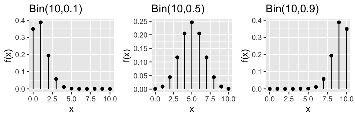
Consider some plots of Binomial RVs for different parameters $n$ and $p$:

In R: Suppose $X \sim Bin(n,p)$…

# Calculate f(x)
dbinom(x, size = n, prob = p)

# Calculate P(X <= x)    
pbinom(x, size = n, prob = p)

# Plot f(x) for x from 0 to n
library(ggplot2)
x <- c(0:n)
binom_data <- data.frame(x = x, fx = dbinom(x, size = n, prob = p))
ggplot(binom_data, aes(x = x, y = fx)) + 
    geom_point()

23.5.2 Discrete Uniform

Suppose discrete RV $X$ is equally likely to be any value in the discrete set $S = \{s_1,s_2,...,s_n\}$. Then $X$ has a discrete uniform model on $S$ with pdf

\[f(x) = P(X=x) = \frac{1}{n} \;\; \text{ for } x \in \{s_1,s_2,...,s_n\}\]

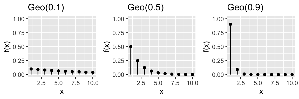
23.5.3 Geometric

Let discrete RV $X$ be the number of trials until the 1st success where:

the trials are independent;
each trial has an equal probability $p$ of success

Then $X$ is Geometric with parameter $p \in (0,1]$:
\[X \sim Geo(p)\] with pdf \[f(x) = P(X=x) = (1-p)^{x-1}p \;\; \text{ for } x \in \{1,2,...\}\]

Properties: \[\begin{split} E(X) & = \frac{1}{p} \\ \text{Mode}(X) & = 1 \\ Var(X) & = \frac{1-p}{p^2} \\ \end{split}\]

Notes:

$f(x) = (\text{probability of $x-1$ failures}) * (\text{probability of 1 success})$
There are other parameterizations of the geometric model. They are used in different ways but produce the same “answer.”

Consider some plots of Geometric RVs for different parameters $p$:

In R: Suppose $X \sim Geo(p)$…

# Calculate f(x)
dgeom(x - 1, prob = p)

# Calculate P(X <= x)    
pgeom(x - 1, prob = p)

# Plot f(x) for x from 1 to m (you pick m)
library(ggplot2)
x <- c(1:m)
geo_data <- data.frame(x = x, fx = dgeom(x-1, prob = p))
ggplot(geo_data, aes(x = x, y = fx)) + 
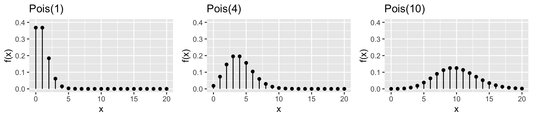
    geom_point()

23.5.4 Poisson

VIDEO: Watch this video for a quick tutorial of the Poisson model.

Let discrete RV $X \in \{0,1,2,...\}$ be the number of events in a given time period. The outcome of $X$ depends upon parameter $\lambda>0$, the rate at which the events occur (ie. the average number of events per time interval). In this setting, we can often model $X$ by a Poisson model: \[X \sim Pois(\lambda)\] with pdf \[f(x) = P(X=x) = \frac{\lambda^x e^{-\lambda}}{x!} \;\; \text{ for } x \in \{0,1,2,...\}\]

Properties: \[\begin{split}E(X) & = \lambda \\ Var(X) & = \lambda \\ \end{split}\] Consider some plots of Poisson RVs for different parameters $\lambda$:

In R: Suppose $X \sim Pois(a)$…

# Calculate f(x)
dpois(x, lambda = a)

# Calculate P(X <= x)    
ppois(x, lambda = a)

# Plot f(x) for x from 0 to m (you choose m)
library(ggplot2)
x <- c(0:m)
pois_data <- data.frame(x = x, fx=dpois(x, lambda = a))
ggplot(pois_data, aes(x = x, y = fx)) + 
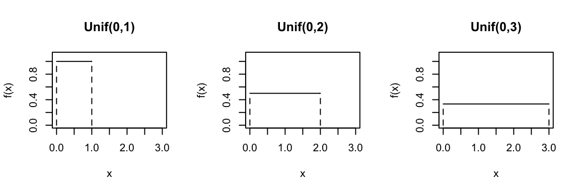
    geom_point()

23.5.5 Continuous Uniform

If continuous RV $X$ is uniformly distributed across the interval $[a,b]$, then

\[X \sim Unif(a,b)\]

with pdf

\[f(x) = \frac{1}{b-a} \;\; \text{ for } x \in [a,b]\]

Properties: \[\begin{split}E(X) & = \frac{a+b}{2} \\ Var(X) & = \frac{(b-a)^2}{12} \\ \end{split}\]

Consider the Uniform model for different parameters $a$ and $b$:

In R: Suppose $X \sim Unif(a,b)$…

# Calculate f(x)
dunif(x, min = a, max = b)

# Calculate P(X <= x)    
punif(x, min = a, max = b)

# Plot f(x) for x from a-1 to b+1 (you pick the range)
ggplot(NULL, aes(x = c(a-1, b+1))) + 
    stat_function(fun = dunif, args = list(min = a, max = b))

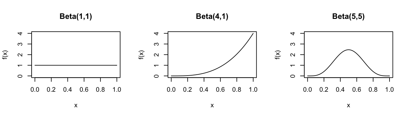
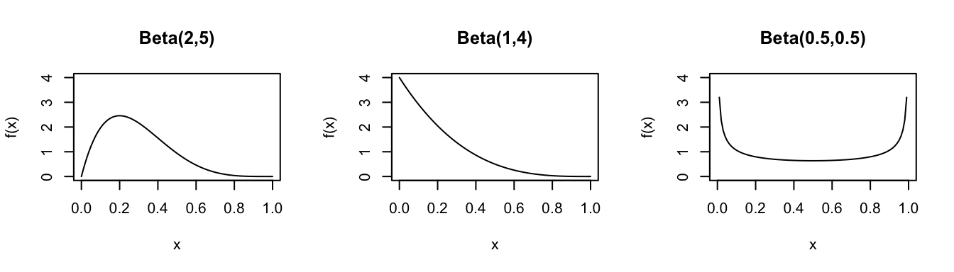
23.5.6 Beta

VIDEO: Watch this video for a quick tutorial of the Beta model.

The Beta model can be used to model a continuous RV $X$ that’s restricted to values in the interval [0,1]. It’s defined by two shape parameters, $\alpha$ and $\beta$:

\[X \sim Beta(\alpha,\beta)\]

with pdf

\[f(x) = \frac{\Gamma(\alpha + \beta)}{\Gamma(\alpha)\Gamma(\beta)} x^{\alpha-1} (1-x)^{\beta-1} \;\; \text{ for } x \in [0,1]\]

NOTE: For positive integers $n$, the gamma function simplifies to $\Gamma(n) = (n-1)!$. Otherwise, $\Gamma(z) = \int_0^\infty x^{z-1}e^{-x}dx$.

Properties: \[\begin{split} E(X) & = \frac{\alpha}{\alpha + \beta} \\ Mode(X) & = \frac{\alpha-1}{\alpha+\beta-2} \\ Var(X) & = \frac{\alpha \beta}{(\alpha + \beta)^2(\alpha+\beta+1)}\\ \end{split}\]

Consider the Beta model for different parameters $\alpha$ and $\beta$:

In R: Suppose $X \sim Beta(a,b)$…

# Calculate f(x)
dbeta(x, shape1 = a, shape2 = b)

# Calculate P(X <= x)    
pbeta(x, shape1 = a, shape2 = b)

# Plot f(x) for x from 0 to m (you pick the range)
ggplot(NULL, aes(x = c(0, m))) + 
    stat_function(fun = dbeta, args = list(shape1 = a, shape2 = b))

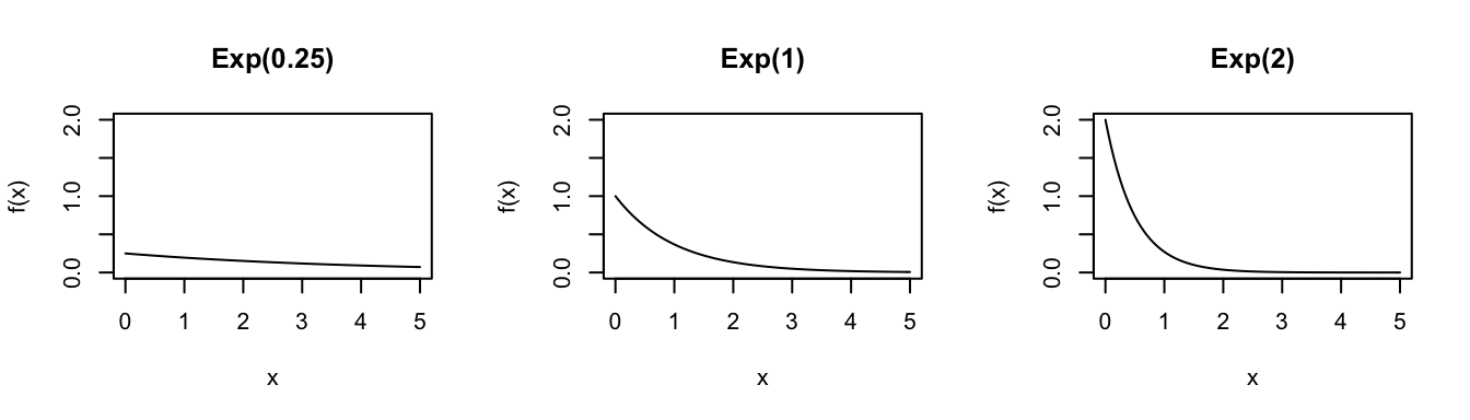
23.5.7 Exponential

Let $X$ be the waiting time until a given event occurs. For example, $X$ might be the time until a lightbulb burns out or the time until a bus arrives. The outcome of $X$ depends upon parameter $\lambda>0$, the rate at which events occur (ie. the number of events per time period). In this scenario, $X$ can often be modeled by an Exponential model: \[X \sim \text{Exp}(\lambda)\]

with pdf \[f(x) = \lambda e^{-\lambda x} \;\; \text{ for } x \in [0,\infty)\]

Properties: \[\begin{split} E(X) & = \frac{1}{\lambda} \\ Var(X) & = \frac{1}{\lambda^2} \\ \end{split}\]

Consider the Exponential model for different parameters $\lambda$:

In R: Suppose $X \sim Exp(a)$…

# Calculate f(x)
dexp(x, rate = a)

# Calculate P(X <= x)    
pexp(x, rate = a)

# Plot of f(x) for x from 0 to m (you pick the range)
ggplot(NULL, aes(x = c(0, m))) + 
    stat_function(fun = dexp, args = list(rate = a))

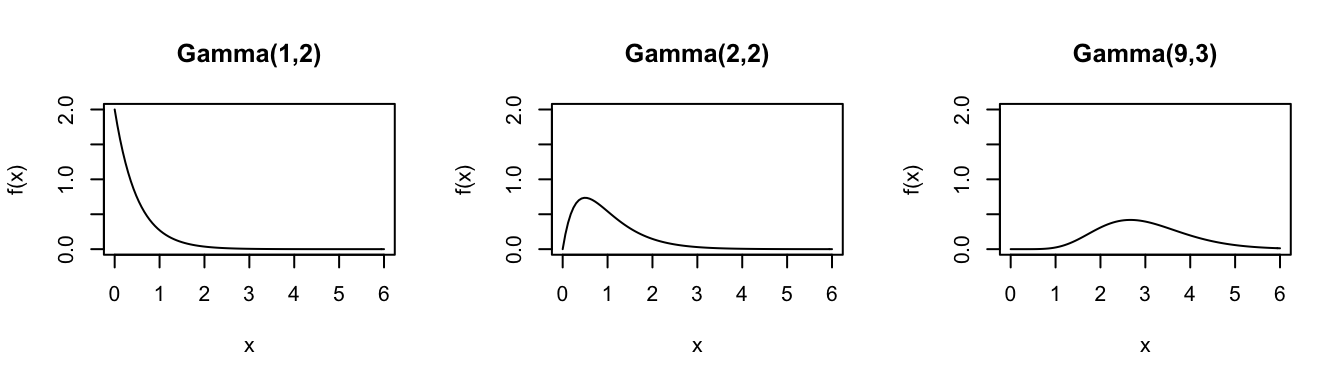
23.5.8 Gamma

VIDEO: Watch this video for a quick tutorial of the Gamma model.

The Gamma model is often appropriate for modeling positive RVs $X$ ($X>0$) with right skew. For example, let $X$ be the waiting time until a given event occurs $s$ times. The outcome of $X$ depends upon both the shape parameter $s>0$ (the number of events we’re waiting for) and the rate parameter $r>0$ (the rate at which the events occur). In this setting, $X$ can often be modeled by a Gamma model: \[X \sim \text{Gamma}(s,r)\]

with pdf \[f(x) = \frac{r^s}{\Gamma(s)}*x^{s-1}e^{-r x} \hspace{.2in} \text{ for } x \in [0,\infty)\] NOTE: For positive integers $s \in \{1,2,...\}$, the gamma function simplifies to $\Gamma(s) = (s-1)!$. Otherwise, $\Gamma(s) = \int_0^\infty x^{s-1}e^{-x}dx$.

Properties: \[\begin{split} E(X) & = \frac{s}{r} \\ Mode(X) & = \frac{s-1}{r} \;\; \text{ (if $s>1$)} \\ Var(X) & = \frac{s}{r^2} \\ \end{split}\]

Consider the Gamma model for different parameters $(s,r)$:

In R: Suppose $X \sim Gamma(s,r)$…

# Calculate f(x)
dgamma(x, shape = s, rate = r)

# Calculate P(X <= x)    
pgamma(x, shape = s, rate = r)

# Plot of f(x) for x from 0 to m (you pick the range)
ggplot(NULL, aes(x = c(0, m))) + 
    stat_function(fun = dgamma, args = list(shape = s, rate = f))

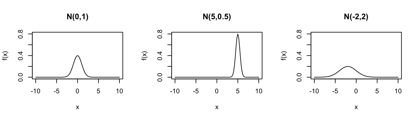
23.5.9 Normal

Let $X$ be an RV with a bell-shaped model centered at $\mu$ and with variance $\sigma^2$. Then $X$ is often well-approximated by a Normal model: \[X \sim \text{Normal}(\mu,\sigma^2)\] with pdf \[f(x) = \frac{1}{\sqrt{2\pi\sigma^2}}*\exp\left\lbrace - \frac{1}{2}\left(\frac{x-\mu}{\sigma} \right)^2 \right\rbrace \hspace{.2in} \text{ for } x \in (-\infty,\infty)\]

Properties: \[\begin{split} E(X) & = \mu \\ Var(X) & = \sigma^2 \\ \end{split}\]

Consider the Normal model for different parameters $(\mu,\sigma^2)$:

In R: Suppose $X \sim N(m,s^2)$…

# Calculate f(x)
dnorm(x, mean = m, sd = s)

# Calculate P(X <= x)    
pnorm(x, mean = m, sd = s)

# Plot f(x) for x from a to b (you pick the range)
ggplot(NULL, aes(x = c(a, b))) + 
    stat_function(fun = dnorm, args = list(mean = m, sd = s))