14 Logistic regression
GOALS
Not all models have quantitative response variables \(Y\). We’ll explore model building and evaluation when \(Y\) is binary (yes/no, pass/fail, etc).
RECOMMENDED READING
Bayes Rules! Chapter 13.
14.1 Warm-up
WARM-UP 1: Just \(Y\)
Suppose we’re interested in identifying whether or not a news article is fake news (vs real news),
\[Y = \begin{cases} 1 & \text{ fake} \\ 0 & \text{ real} \\ \end{cases}\]
What’s an appropriate model for the variability in \(Y_i\) from article to article?
- \(Y_i | \pi \stackrel{ind}{\sim} \text{Bin}(1, \pi)\), i.e. \(Y_i | \pi \stackrel{ind}{\sim} \text{Bern}(\pi)\) with \(E(Y_i | \pi) = \pi\)
- \(Y_i | \lambda \stackrel{ind}{\sim} \text{Pois}(\lambda)\) with \(E(Y_i | \lambda) = \lambda\)
- \(Y_i | \mu, \sigma \stackrel{ind}{\sim} N(\mu, \sigma^2)\) with \(E(Y_i | \mu, \sigma) = \mu\)
WARM-UP 2: Finish the Bayesian model
Suppose we wished to predict whether an article is fake (\(Y\)) based on its title alone. For example:
- “President’s approval rating at a new low”
- “The president has a funny secret and doesn’t want you to know about it!”
Consider just two possible metrics: the number of words in the title (\(X_1\)) and whether the title has an exclamation point (\(X_2\)). Modify your model from the first warm-up example to build out the regression model of \(Y\) vs \(X_1\) and \(X_2\). In doing so, think carefully about:
What function of \(E(Y_i|X) = \pi_i\) we’ll assume to be linearly dependent on the predictors. That is, what’s an appropriate \(g()\)?
\[g(\pi_i) = \beta_0 + \beta_1 X_{i1} + \beta_2 X_{i2}\]Priors.
The Bayesian logistic regression model
To model binary response variable \(Y \in \{0, 1\}\) by predictor \(X\), suppose we collect \(n\) data points. Let \((Y_i, X_i)\) denote the observed data on each case \(i \in \{1, 2, \ldots, n\}\). Then the Bayesian logistic regression model is as follows:
\[\begin{array}{rll} Y_i | \beta_0, \beta_1, \sigma & \stackrel{ind}{\sim} \text{Bern}(\pi_i) & \text{where } \log\left(\frac{\pi_i}{1 - \pi_i}\right) = \beta_0 + \beta_1 X_i \\ && \text{equivalently, } \frac{\pi_i}{1 - \pi_i} = e^{\beta_0 + \beta_1 X_i} \; \text{ and } \pi_i = \frac{e^{\beta_0 + \beta_1 X_i}}{e^{\beta_0 + \beta_1 X_i} + 1}\\ \beta_{0c} & \sim N(m_0, s_0^2) & \\ \beta_1 & \sim N(m_1, s_1^2) & \\ \end{array}\]
NOTES:
The priors on \((\beta_0, \beta_1)\) are independent of one another.
For interpretability, we state our prior understanding of the model intercept \(\beta_0\) through the centered intercept \(\beta_{0c}\).
When \(X = 0\), \(\beta_0\) is the expected logged odds for the event of interest and \(e^{\beta_0}\) is the expected odds.
For each 1-unit increase in \(X\), \(\beta_1\) is the expected change in the logged odds of the event of interest and \(e^{\beta_1}\) is the expected multiplicative change in odds. That is
\[\beta_1 = \log(\text{odds}_{x+1}) - \log(\text{odds}_x) \;\; \text{ and } \;\; e^{\beta_1} = \frac{\text{odds}_{x+1}}{\text{odds}_x}\]
14.2 Exercises
NOTE
These exercises focus on new concepts. They do not reflect the entire Bayesian modeling workflow.
THE STORY
The fake_news dataset includes information on 150 different news articles that were posted to Facebook, some real some fake. You’ll use this data to model and classify whether an article is_fake \(Y\) by its number of title_words \(X_1\) and title_has_excl \(X_2\) (whether the title includes an exclamation point).
# Load packages
library(tidyverse)
library(tidybayes)
library(rstan)
library(rstanarm)
library(bayesplot)
library(bayesrules)
library(broom.mixed)

# Load data
fake_news <- read.csv("https://www.macalester.edu/~ajohns24/data/fake_news.csv") %>%
  mutate(is_fake = (type == "fake"))
We’ll start with the following logistic regression model where we’ll use weakly informative priors:
\[\begin{array}{rll} Y_i | \beta_0, \beta_1, \beta_2 \sigma & \stackrel{ind}{\sim} \text{Bern}(\pi_i) & \text{where } \log\left(\frac{\pi_i}{1 - \pi_i}\right) = \beta_0 + \beta_1 X_{i1} + \beta_2 X_{i2} \\ && \text{equivalently, } \frac{\pi_i}{1 - \pi_i} = e^{\beta_0 + \beta_1 X_{i1} + \beta_2 X_{i2}} \; \text{ and } \pi_i = \frac{e^{\beta_0 + \beta_1 X_{i1} + \beta_2 X_{i2}}}{e^{\beta_0 + \beta_1 X_{i1} + \beta_2 X_{i2}} + 1}\\ \beta_{0c} & \sim N(m_0, s_0^2) & \\ \beta_1 & \sim N(m_1, s_1^2) & \\ \beta_2 & \sim N(m_2, s_2^2) & \\ \end{array}\]
14.2.1 Part 1: Simulate and analyze the model
- Check out the data
Since response variableis_fakeis categorical, visualizing the data in a logistic regression setting is different than for Normal or Poisson regression. Code is provided.Construct and interpret a jitter plot of
is_fakeversustitle_wordsandtitle_has_excl:ggplot(fake_news, aes(x = title_words, y = is_fake, color = title_has_excl)) + geom_jitter(height = 0.25)To learn more about the relationship between
is_fakeandtitle_words, we can calculate the proportion of articles that are fake in each of severaltitle_wordsbrackets. For example, for articles with between 5 and 8 words in the title, what proportion are fake? What about articles with between 19 and 22 words in the title?# Calculate the fake news rate by title words bracket bracketed_data <- fake_news %>% mutate(word_bracket = cut(title_words, breaks = 5)) %>% group_by(word_bracket) %>% summarize(fake_rate = mean(is_fake)) bracketed_data ## # A tibble: 5 x 2 ## word_bracket fake_rate ## <fct> <dbl> ## 1 (4.98,8.4] 0.278 ## 2 (8.4,11.8] 0.283 ## 3 (11.8,15.2] 0.561 ## 4 (15.2,18.6] 0.588 ## 5 (18.6,22] 0.667Plot and summarize a scatterplot of
fake_rate(y-axis) vsword_bracket(x-axis). NOTE: addingtheme(axis.text.x = element_text(angle = 45, vjust = 0.5))will make it easier to read the x-axis.
Simulate the posterior model
Change ONE LINE in the code below to simulate the posterior logistic regression model.# Simulate the posterior logistic regression model logistic_model_1 <- stan_glm( is_fake ~ title_words + title_has_excl, data = fake_news, family = gaussian, chains = 4, iter = 5000*2, seed = 84735, refresh = 0)
Plot the posterior model
Check out the plot below of 100 different posterior scenarios for our relationship of interest. Use this to summarize our posterior understanding and comment on whether this understanding is strong or weak.fake_news %>% add_fitted_draws(logistic_model_1, n = 100) %>% ggplot(aes(x = title_words, y = is_fake, color = title_has_excl)) + geom_line(aes(y = .value, group = paste(title_has_excl, .draw)), alpha = 0.5) + labs(y = "probability that article is fake")
- Posterior estimation
Construct a
tidy()summary of the posterior model, including 80% credible intervals.
How can we interpret the posterior median estimate of the
title_wordscoefficient:\[\beta_1 = 0.144 \;\; \text{ and } e^{\beta_1} = 1.15\]
When controlling for whether or not the title has an exclamation point, for each additional word in the title…
- the log(odds) that the article is fake increase by 1.15.
- the odds that the article is fake increase by 1.15.
- the odds that the article is fake increase by 15% (i.e. multiply by 1.15).
- the probability that the article is fake increase by 15% (i.e. multiply by 1.15.
How can we interpret the posterior median estimate of the
title_has_exclTRUEcoefficient:\[\beta_2 = 2.81 \;\; \text{ and } e^{\beta_2} = 16.6\]
When controlling for the number of words in the title, if the title has an exclamation point…
- the odds that the article is fake are 16.6 greater than the odds that it’s real.
- the odds that the article is fake are 16.6 times greater than the odds that it’s real.
- the probability that the article is fake is 16.6 greater than the probability that it’s real.
- the probability that the article is fake is 16.6 times greater than the probability that it’s real.
- the odds that the article is fake are 16.6 greater than the odds that it’s real.
Do we have ample evidence that, when controlling for the other predictor in the model, both the number of words in the title and whether the title has an exclamation point are significantly associated with whether the article is fake?
Posterior prediction & classification
Suppose we come across an article on Facebook that has 20 words but no exclamation point in the title. We can simulate a posterior predictive model for the fake / real status of this article usingposterior_predict():# Simulate the posterior predictive model set.seed(84735) binary_prediction <- posterior_predict( logistic_model_1, newdata = data.frame(title_words = 20, title_has_excl = FALSE))Check out the visual and numerical summaries of this posterior predictive model. What’s the posterior probability that the article is fake?
# Plot the posterior predictive model mcmc_hist(binary_prediction) + labs(x = "Y") # Numerical summary of predictive model table(binary_prediction)If you had to make a yes-or-no classification of whether or not this particular article is fake, what would you say: fake or real? Why?
In making your classification in part b, what classification rule are you using: Since the probability of being fake > _____, classify as fake.
EXTRA PRACTICE: After class, simulate the posterior predictive model from scratch, without using the
posterior_predict()function.
14.2.2 Part 2: Evaluate the model
Just as with Normal and Poisson regression, we must evaluate the quality of our logistic regression model before going any further.
- Is the model fair?
- How wrong is the model?
Construct and interpret a
pp_check(). This plots the proportion of fake and real news in each of 50 posterior simulated datasets, alongside the observed proportion of fake and real news in our sampled articles.The
pp_check()is a little goofy in the logistic regression context. To better visualize if our posterior model reflects the observed proportion of news articles that are fake, run the code below. How does the fake vs real breakdown in our simulated datasets compare to that in our observed sample?proportion_fake <- function(x){mean(x == 1)} pp_check(logistic_model_1, plotfun = "stat", stat = "proportion_fake") + xlab("proportion that are fake")
How accurate are the posterior classifications? Sensitivity, specificity, and overall accuracy
Our third model evaluation question addresses the accuracy of our posterior news classifications. We’ll start with the following classification rule which uses a probability cut-off of 0.5: If the posterior probability that an article is fake exceeds 0.5, then classify it as fake. Otherwise, classify it as real. Theclassification_summary()function, similar to theprediction_summary()function for Normal and Poisson regression, summarizes the performance and quality of this posterior classification rule:set.seed(84735) classification_summary( model = logistic_model_1, data = fake_news, cutoff = 0.5)The overall accuracy of our posterior classifications reflects the overall proportion of news articles that we correctly classified. Report the
overall_accuracyand confirm how this was calculated from theconfusion_matrix.The specificity of our posterior classifications reflects the overall proportion of real news articles that we correctly classified as real (i.e. the proportion of \(Y = 0\) outcomes that we correctly predicted to be 0). Report the
specificityvalue and confirm how this was calculated from theconfusion_matrix.The sensitivity of our posterior classifications reflects the overall proportion of fake news articles that we correctly classified as fake (i.e. the proportion of \(Y = 1\) outcomes that we correctly predicted to be 1). Report the
sensitivityvalue and confirm how this was calculated from theconfusion_matrix.
How accurate are the posterior classifications? Changing the probability cut-off
Our posterior classifications did a pretty good job of detecting real news articles, but missed a lot of fake news (the consequences being that we’d read a lot of fake news without realizing it).No problem. If we want to catch more fake news, we can simply change the probability cut-off we use in our classification rule. That is, we needn’t compare the posterior probabilities to 0.5. Play around with the
classification_summary()function. Identify a new probabilitycutoffthat catches at least 2/3 of fake news while maintaining as high of specificity as possible (i.e. still does a good job of detecting real news).set.seed(84735) classification_summary( model = logistic_model_1, data = fake_news, cutoff = 0.5)In general, what happens to the specificity of our posterior classifications (our ability to detect real news) as we increase the sensitivity (our ability to detect fake news)?
The importance of sensitivity vs specificity depends upon the context of our analysis. In the fake news context, what’s more important to you, sensitivity (detecting fake news) or specificity (detecting real news)? Think: what are the consequences to increasing sensitivity at the cost of specificity? what are the consequences to increasing specificity at the cost of sensitivity?
How accurate are the posterior classifications? Cross-validation
Finally, the posterior classification summaries above evaluate our model using the same articles we used to build it. Using the cut-off you determined in the exercise above, complement these results using cross-validated classification summaries. NOTE: This takes a while. Because of this, we could continue to tweak our probability cut-off, but won’t.#set.seed(84735) #classification_summary_cv( # model = logistic_model_1, data = fake_news, # cutoff = ___, # k = 10)
- Build a new model
There are lots of other predictors in thefake_newsdata, includingtext_syllables_per_wordand measures on sentiments such asanger,fearandjoy.- Simulate a new posterior model of
is_fake ~ title_words + title_has_excl + text_syllables_per_word + anger + anticipation + disgust + fear + joy + sadness + surprise + trust. Name thislogistic_model_2.
- Which model has the better NON-cross-validated classification performance, the new model or the original model? For comparison purposes, use a 0.5 probability cut-off.
- Which model has the better cross-validated classification performance, the new model or the original model? For comparison purposes, use a 0.5 probability cut-off.
- Which model do you pick?
- Simulate a new posterior model of
Pick a model
We’ve now seen 4 different regression models: Normal, Poisson, Negative Binomial, and logistic. For each of the following situations, identify which would be an appropriate model. Better yet, simulate and run app_check()to support your answer.- Use the
airbnb_smalldata inbayesrulesto model the number ofreviewsan AirBnB listing has by itsrating,district,room_type, and the number of guests itaccommodates. - Use the
hotel_bookingsdata inbayesrulesto model whether a hotel bookingis_canceledbased on thelead_time(how far in advance the booking was made), how manyprevious_cancellationsthe guest has, whether or not the guestis_repeated_guest, and theaverage_daily_rateat the hotel. - Use the
weather_australiadata inbayesrulesto model today’shumidity3pmbased onlocationand whether there wasraintoday.
- Use the
- OPTIONAL: Model selection
Picking a final model isn’t always easy. There are some additional tools that can help. We won’t elaborate on these in class, but they might come in handy for capstones.Beyond comparing cross-validated classification (or prediction) summaries, we can compare models’ classification accuracies using their expected log-predictive densities (ELPD). This is more technical but makes a clearer comparison of two models. In general, the higher the ELPD, the better our posterior model is at predicting / classifying new data points. More technically, ELPD measures the typical log posterior predictive pdf, \(\log(f(y_{new} | y))\). The higher a new value’s log posterior predictive pdf, the more consistent it was with its posterior predictive model.
# Calculate the ELPD for our 2 models model_1_elpd <- loo(logistic_model_1) model_2_elpd <- loo(logistic_model_2) # Compare the ELPD for our 2 models loo_compare(model_1_elpd, model_2_elpd)NOTE: The
loo_compareoutput lists the models from best to worst, i.e. from the highest ELPD to the lowest. Further, it reports the difference in the ELPDs with a corresponding standard error.- Which model has the highest / best ELPD?
- Is its ELPD more than 2 standard errors above the other model’s ELPD? If so, its posterior classifications are “significantly better.” If not, then we might pick whichever is the simpler model.
- Which model has the highest / best ELPD?
If you’ve taken STAT 253, you’ve learned about the LASSO shrinkage method. This method can help narrow down a large set of possible predictors, while making the model more stable / less variable. Not only is there a Bayesian LASSO counterpart, we can achieve a similar effect using horseshoe priors. Do some digging on what a horseshoe prior is and how we might implement horseshoe priors (instead of Normal priors) for our regression coefficients in
stan_glm().
14.3 Solutions
- Check out the data
It appears that fake articles tend to have longer titles and more exclamation marks.
ggplot(fake_news, aes(x = title_words, y = is_fake, color = title_has_excl)) +
  geom_jitter(height = 0.25)
Among articles with between 5 and 8 words in the title, 27.8% are fake. Among articles with between 19 and 22 words in the title, 2/3 are fake.
# Calculate the fake news rate by title words bracket bracketed_data <- fake_news %>% mutate(word_bracket = cut(title_words, breaks = 5)) %>% group_by(word_bracket) %>% summarize(fake_rate = mean(is_fake)) bracketed_data ## # A tibble: 5 x 2 ## word_bracket fake_rate ## <fct> <dbl> ## 1 (4.98,8.4] 0.278 ## 2 (8.4,11.8] 0.283 ## 3 (11.8,15.2] 0.561 ## 4 (15.2,18.6] 0.588 ## 5 (18.6,22] 0.667The probability of an article being fake increases with the number of words in the title.
ggplot(bracketed_data, aes(y = fake_rate, x = word_bracket)) + geom_point()
Simulate the posterior model
# Simulate the posterior logistic regression model logistic_model_1 <- stan_glm( is_fake ~ title_words + title_has_excl, data = fake_news, family = binomial, chains = 4, iter = 5000*2, seed = 84735, refresh = 0)
Plot the posterior model
We have a weak posterior understanding that the probability an article is fake increases with the number of words in its title and if it has exclamation points in the title.fake_news %>% add_fitted_draws(logistic_model_1, n = 100) %>% ggplot(aes(x = title_words, y = is_fake, color = title_has_excl)) + geom_line(aes(y = .value, group = paste(title_has_excl, .draw)), alpha = 0.5) + labs(y = "probability that article is fake")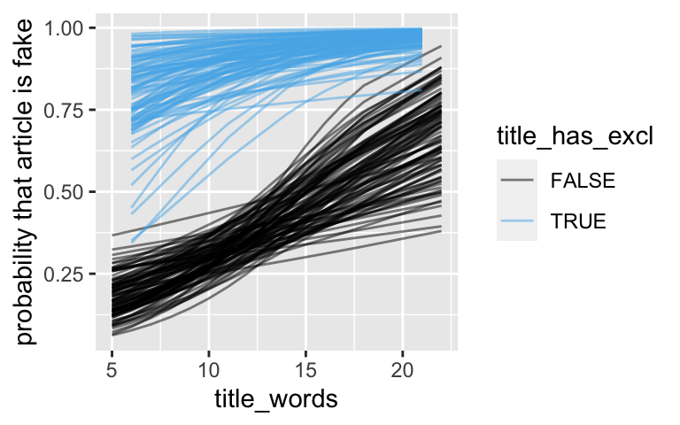
- Posterior estimation
.
tidy(logistic_model_1, conf.int = TRUE, conf.level = 0.8) ## # A tibble: 3 x 5 ## term estimate std.error conf.low conf.high ## <chr> <dbl> <dbl> <dbl> <dbl> ## 1 (Intercept) -2.30 0.660 -3.17 -1.47 ## 2 title_words 0.144 0.0555 0.0738 0.218 ## 3 title_has_exclTRUE 2.81 0.822 1.86 4.03the odds that the article is fake increase by 15% (i.e. multiply by 1.15)
the odds that the article is fake are 16.6 times greater than the odds that it’s real.
Yes, the 80% CIs for the related coefficients (\(\beta_1\) and \(\beta_2\)) are above 0.
Posterior prediction & classification
# Simulate the posterior predictive model set.seed(84735) binary_prediction <- posterior_predict( logistic_model_1, newdata = data.frame(title_words = 20, title_has_excl = FALSE))There’s a 63.44% posterior chance that this article is fake.
# Plot the posterior predictive model mcmc_hist(binary_prediction) + labs(x = "Y")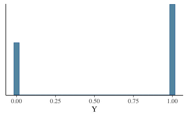
# Numerical summary of predictive model table(binary_prediction) ## binary_prediction ## 0 1 ## 7312 12688 12688/(7312 + 12688) ## [1] 0.6344Answers might vary. Since it’s more likely than not, we might classify it as fake.
Answers might vary. Since the probability of being fake > 0.5, classify as fake.
First get 20,000 equations for the probability that the article is fake, and then simulate a Binomial outcome from each of these possibilities.
set.seed(84735) prediction_scratch <- as.data.frame(logistic_model_1) %>% mutate(logodds = `(Intercept)` + title_words*20) %>% mutate(odds = exp(logodds)) %>% mutate(prob = odds / (odds + 1)) %>% mutate(y_new = rbinom(20000, size = 1, prob = prob)) prediction_scratch %>% count(y_new) ## y_new n ## 1 0 7312 ## 2 1 12688
- Is the model fair?
We should be careful when applying this model. We’d want to be careful that our own biases aren’t baked into our determination of whether an article is real or not. For example, we might consider other possible predictors.
- How wrong is the model?
.
pp_check(logistic_model_1)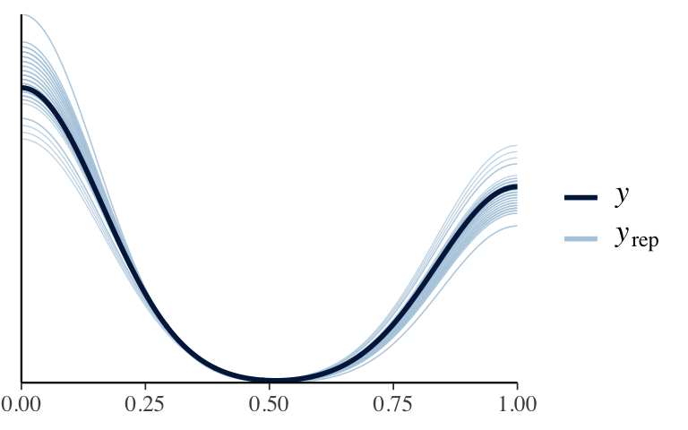
Roughly 40% of the articles in our sample are fake. The proportion in our simulated datasets center at 40% and range from 25% to 55%. Thus our posterior model doesn’t seem to wrong (though it’s maybe weak).
proportion_fake <- function(x){mean(x == 1)}
pp_check(logistic_model_1,
         plotfun = "stat", stat = "proportion_fake") +
  xlab("proportion that are fake")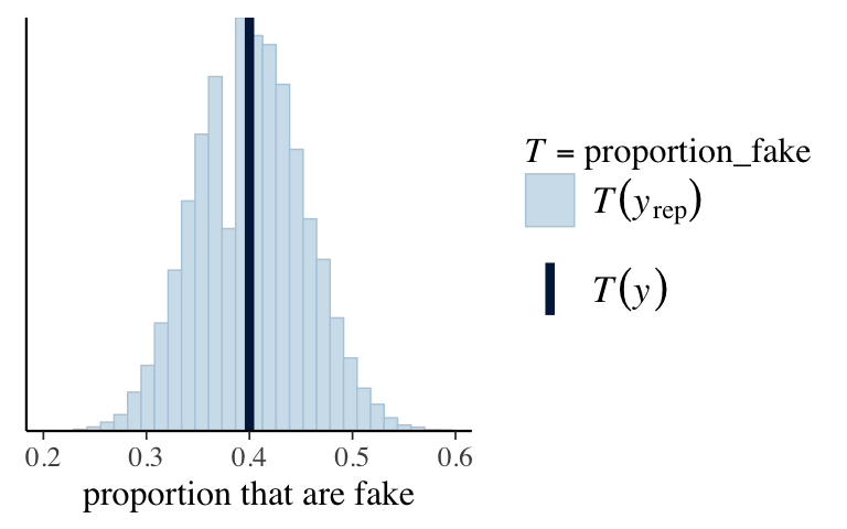
How accurate are the posterior classifications? Sensitivity, specificity, and overall accuracy
set.seed(84735) classification_summary( model = logistic_model_1, data = fake_news, cutoff = 0.5) ## $confusion_matrix ## y 0 1 ## FALSE 81 9 ## TRUE 39 21 ## ## $accuracy_rates ## ## sensitivity 0.35 ## specificity 0.90 ## overall_accuracy 0.68# a. overall accuracy (81 + 21) / (81 + 21 + 9 + 39) ## [1] 0.68 # b. specificity 81 / (81 + 9) ## [1] 0.9 # c. sensitivity 21 / (21 + 39) ## [1] 0.35
- How accurate are the posterior classifications? Changing the probability cut-off
A cut-off of 0.36, i.e. classifying an article as fake if it has even a 36% chance of being fake, catches 2/3 of fake news and 72.2% of real news.
set.seed(84735) classification_summary( model = logistic_model_1, data = fake_news, cutoff = 0.36) ## $confusion_matrix ## y 0 1 ## FALSE 65 25 ## TRUE 20 40 ## ## $accuracy_rates ## ## sensitivity 0.6666667 ## specificity 0.7222222 ## overall_accuracy 0.7000000as sensitivity increases, specificity decreases (there’s a trade-off!)
will vary. there are consequences to both answers.
How accurate are the posterior classifications? Cross-validation
set.seed(84735) classification_summary_cv( model = logistic_model_1, data = fake_news, cutoff = 0.36, k = 10) ## $folds ## fold sensitivity specificity overall_accuracy ## 1 1 0.8000000 0.5000000 0.6000000 ## 2 2 0.4000000 0.8000000 0.6666667 ## 3 3 0.6666667 0.8333333 0.7333333 ## 4 4 0.6250000 0.7142857 0.6666667 ## 5 5 0.7142857 1.0000000 0.8666667 ## 6 6 0.4285714 0.7500000 0.6000000 ## 7 7 0.8000000 1.0000000 0.9333333 ## 8 8 0.6666667 0.8333333 0.8000000 ## 9 9 0.7142857 0.7500000 0.7333333 ## 10 10 0.5000000 0.5454545 0.5333333 ## ## $cv ## sensitivity specificity overall_accuracy ## 1 0.6315476 0.7726407 0.7133333
- Build a new model
.
# Simulate the posterior logistic regression model logistic_model_2 <- stan_glm( is_fake ~ title_words + title_has_excl + text_syllables_per_word + anger + anticipation + disgust + fear + joy + sadness + surprise + trust, data = fake_news, family = binomial, chains = 4, iter = 5000*2, seed = 84735, refresh = 0)Model 2 has the better NON-cross-validated sensitivity and overall accuracy.
set.seed(84735) classification_summary( model = logistic_model_1, data = fake_news, cutoff = 0.5) ## $confusion_matrix ## y 0 1 ## FALSE 81 9 ## TRUE 39 21 ## ## $accuracy_rates ## ## sensitivity 0.35 ## specificity 0.90 ## overall_accuracy 0.68 set.seed(84735) classification_summary( model = logistic_model_2, data = fake_news, cutoff = 0.5) ## $confusion_matrix ## y 0 1 ## FALSE 78 12 ## TRUE 27 33 ## ## $accuracy_rates ## ## sensitivity 0.5500000 ## specificity 0.8666667 ## overall_accuracy 0.7400000Model 2 has the better cross-validated sensitivity, but lower specificity and overall accuracy.
set.seed(84735) classification_summary_cv( model = logistic_model_1, data = fake_news, cutoff = 0.5, k = 10) ## $folds ## fold sensitivity specificity overall_accuracy ## 1 1 0.6000000 0.5000000 0.5333333 ## 2 2 0.4000000 1.0000000 0.8000000 ## 3 3 0.2222222 1.0000000 0.5333333 ## 4 4 0.3750000 0.8571429 0.6000000 ## 5 5 0.1428571 1.0000000 0.6000000 ## 6 6 0.2857143 0.8750000 0.6000000 ## 7 7 0.2000000 1.0000000 0.7333333 ## 8 8 0.3333333 1.0000000 0.8666667 ## 9 9 0.5714286 0.8750000 0.7333333 ## 10 10 0.2500000 0.9090909 0.7333333 ## ## $cv ## sensitivity specificity overall_accuracy ## 1 0.3380556 0.9016234 0.6733333 set.seed(84735) classification_summary_cv( model = logistic_model_2, data = fake_news, cutoff = 0.5, k = 10) ## $folds ## fold sensitivity specificity overall_accuracy ## 1 1 0.4000000 0.6000000 0.5333333 ## 2 2 0.2000000 0.8000000 0.6000000 ## 3 3 0.4444444 0.8333333 0.6000000 ## 4 4 0.5000000 0.5714286 0.5333333 ## 5 5 0.2857143 0.8750000 0.6000000 ## 6 6 0.2857143 1.0000000 0.6666667 ## 7 7 0.4000000 1.0000000 0.8000000 ## 8 8 0.6666667 0.8333333 0.8000000 ## 9 9 0.5714286 0.6250000 0.6000000 ## 10 10 0.2500000 1.0000000 0.8000000 ## ## $cv ## sensitivity specificity overall_accuracy ## 1 0.4003968 0.8138095 0.6533333Tough call! We should dig in deeper. For example, we might compare both at the “optimal” probability cut-off. I’d probably go with the simpler model.
- Pick a model
You might explore similar questions on the next homework.
- OPTIONAL: Model selection
Model 1 has the higher / better ELPD – it’s 4.9 units above the ELPD for Model 2. Model 2’s ELPD is within 2 standard errors, i.e. 0 is within the realm of possible differences: \(4.9 \pm 2*4.1 = (-3.3, 13.1)\). Thus the posterior classification quality is not significantly different for the 2 models. In this case, I’d pick the simpler model 1.
# Calculate the ELPD for our 2 models model_1_elpd <- loo(logistic_model_1) model_2_elpd <- loo(logistic_model_2) # Compare the ELPD for our 2 models loo_compare(model_1_elpd, model_2_elpd) ## elpd_diff se_diff ## logistic_model_1 0.0 0.0 ## logistic_model_2 -4.9 4.1general info about horseshoe priors
horseshoe priors in stan_glm