7 Posterior estimation & hypothesis testing
GOALS
We’ve learned how to build Bayesian models and to approximate Bayesian models using Markov chain Monte Carlo (MCMC) techniques. Now let’s use these models to “say something” or make inferences about our parameter of interest, “\(\pi\).” The following are key steps:
- estimation
obtain a single posterior point estimate of \(\pi\) as well as a range of posterior plausible values - hypothesis testing
use the posterior to assess a claim about \(\pi\) - prediction
use the posterior to predict a new observation of \(Y\)
RECOMMENDED READING
Bayes Rules! Chapter 8.
7.1 R code reference
# Handy packages
library(bayesrules)
library(rstan)
library(rstanarm)
library(bayesplot)
library(broom.mixed)
Exact properties of a Beta model
# Calculate the mean, mode, and sd of a Beta(a,b) model
summarize_beta(alpha = a, beta = b)

# Calculate the qth quantile of a Beta(a,b) where q is btwn 0 and 1
qbeta(q, shape1 = a, shape2 = b)

# Calculate the probability that a Beta(a,b) variable is below c
pbeta(c, shape1 = a, shape2 = b)
Calculating properties of a sample
Let data be a data frame and x be a variable within the data.
# Calculate the mean x value
data %>%
  summarize(mean(x))

# Calculate the qth quantile of x values where q is btwn 0 and 1
data %>%
  summarize(quantile(x, q))

# Calculate the proportion of x values that fall below c
data %>%
  summarize(mean(x < c))
Summarizing the properties of an MCMC simulation
Let model_sim be our simulation results.
# Calculate the posterior median and 95% posterior credible intervals
# (You can change 95%)
tidy(model_sim, conf.int = TRUE, conf.level = 0.95)

# Plot the posterior approximation and
# Shade in the 95% posterior credible interval
mcmc_areas(model_sim, pars = "pi", prob = 0.95)

# Store the simulation results in a data frame that
# can be summarized in the tidyverse
model_chains <- as.data.frame(model_sim, pars = "lp__", include = FALSE)
model_chains %>%
  summarize(___)
7.2 Warm-up
Let \(\pi \in [0,1]\) be the proportion of U.S. adults that don’t believe in climate change. To learn about \(\pi\), we’ll start with a Beta(1,2) prior and survey 1000 adults and record \(Y\), the number that don’t believe in climate change:
# Load packages and data
library(bayesrules)
library(tidyverse)
data("pulse_of_the_nation")

# Count up the number that don't believe in climate change
pulse_of_the_nation %>%
  count(climate_change)
## # A tibble: 3 x 2
##   climate_change                    n
##   <fct>                         <int>
## 1 Not Real At All                 150
## 2 Real and Caused by People       655
## 3 Real but not Caused by People   195
Thus we have the following model:
\[\begin{split} Y|\pi & \sim Bin(1000,\pi) \\ \pi & \sim Beta(1, 2) \\ \end{split} \;\; \Rightarrow \;\; \pi | (Y = 150) \sim Beta(151, 852)\]
plot_beta_binomial(alpha = 1, beta = 2, y = 150, n = 1000)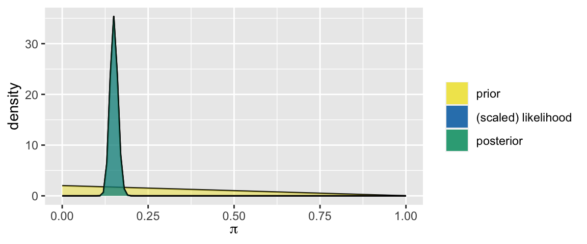
Bayesian vs frequentist inference
In a frequentist analysis, \(\pi\) is viewed as a fixed, unknown quantity. We make inferences about \(\pi\) using data \(Y\).
In a Bayesian analysis, \(\pi\) is viewed as a random variable. We make inferences about \(\pi\) using the posterior, which combines the prior and data \(Y\).
EXAMPLE: A quick frequentist analysis
- What’s the frequentist estimate of \(\pi\)?
Let \(\overline{y} = 150/1000 = 0.15\). Then the 95% frequentist confidence interval for \(\pi\) is
\[\overline{y} \pm 1.96 \sqrt{\frac{\overline{y}(1-\overline{y})}{1000}} = 0.15 \pm 0.02 = (0.13, 0.17)\]
How can we interpret this?
- There’s a 95% chance that \(\pi\) is between 0.13 and 0.17: \[P(\pi \in (0.13, 0.17) | \overline{y} = 0.15) = 0.95\]
- There’s a 95% chance that the survey results we happened to get produced an interval that covers \(\pi\): \[P\left(\overline{Y} \in (\pi - 0.02, \pi + 0.02)\right) = 0.95\]
- There’s a 95% chance that \(\pi\) is between 0.13 and 0.17: \[P(\pi \in (0.13, 0.17) | \overline{y} = 0.15) = 0.95\]
The frequentist p-value for the hypothesis test of \(H_0: \pi = 0.13\) vs \(H_a: \pi > 0.13\) is 0.033. How can we interpret this?
- \(P(\pi > 0.13 | \overline{y} = 0.15)\): Given our polling results, there’s a 3.3% chance that \(\pi\) exceeds 0.13.
- \(P(\overline{Y} \ge 0.15 | \pi = 0.13)\): If in fact \(\pi\) were only 0.13, there’s a 3.3% chance that we would’ve gotten a survey in which 15% or more didn’t believe in climate change.
- \(P(\pi > 0.13 | \overline{y} = 0.15)\): Given our polling results, there’s a 3.3% chance that \(\pi\) exceeds 0.13.
- How were the confidence interval and p-value calculated?
7.3 Exercises
OK. That was weird. In contrast, the Bayesian approach is quite natural. It also only requires the posterior model, so once we’ve done that work we have everything we need! In the exercises below, you’ll challenge yourself to perform a Bayesian posterior analysis without being given any formulas or direction. (You can do it.) You’ll take two approaches:
- an exact analysis utilizing the known Beta(151, 852) posterior;
- an approximate analysis utilizing an MCMC simulation of the Beta(151, 852) posterior.
NOTE:
- Pause and discuss each exercise with your group. Support one another in trying out new ideas. Practice discussing Bayesian concepts.
- Do NOT use any frequentist formulas in your Bayesian analysis. Rely on the posterior properties alone.
7.3.1 An exact analysis
Bayesian estimation
Bayesians think of the entire Beta(151,852) posterior pdf as an estimate for \(\pi\). But for communication purposes, it can be useful to estimate what values of \(\pi\) are typical. Identify and calculate two possible posterior point estimates, i.e. single possible values of \(\pi\). NOTE: Checking out a plot of the posterior might spark some ideas, and formulas for the general Beta properties will come in handy.plot_beta(151, 852) + xlim(0.1, 0.2)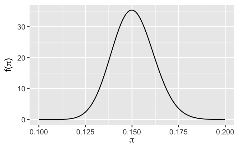
Bayesian interval estimation
The posterior estimates above merely capture the typical posterior \(\pi\) value, thus miss the bigger picture. It’s important to supplement these estimates with a posterior credible interval. NOTE: Bayesians use “credible” intervals whereas frequentists use “confidence” intervals.Calculate a 95% posterior credible interval for \(\pi\). Revisiting a plot of the Beta(151,852) posterior might spark some ideas. NOTE: You’ll need some R code.
How can we interpret this interval, (a,b)?
- There’s a 95% posterior probability that \(\pi\), the proportion of people that don’t believe in climate change, is between a and b: \(P(\pi \in (a, b) | Y = 150) = 0.95\)
- There’s a 95% posterior probability that the survey results we happened to get produced an interval that covers \(\pi\): \(P\left(\frac{Y}{n} \in (\pi - (b-a)/2, \pi + (b-a)/2)\right) = 0.95\)
- There’s a 95% posterior probability that \(\pi\), the proportion of people that don’t believe in climate change, is between a and b: \(P(\pi \in (a, b) | Y = 150) = 0.95\)
Ask a (strict) frequentist: What’s the probability that \(\pi\) lies within the Bayesian credible interval?
Bayesian hypothesis testing
A researcher claims that more than 13% of people don’t believe in climate change. Let’s assess this claim holistically.Check out the posterior model. Using this graphical tool alone, what do you think about this claim?
plot_beta(151, 852) +
  xlim(0.1, 0.2)
Recall your credible interval for \(\pi\) from the previous example. Using this interval, what do you think about this claim?
Calculate and interpret a posterior probability that helps you test this claim. NOTE: You’ll need some R code.
How can we interpret this posterior probability?
- \(P(\pi > 0.13 | \overline{y} = 0.15)\): Given our polling results, this is the probability that the claim is correct.
- \(P(\overline{Y} \ge 0.15 | \pi = 0.13)\): If in fact \(\pi\) were only 0.13, this is the chance we would’ve gotten a survey in which 15% or more didn’t believe in climate change.
There’s no common cut-off / threshold (eg: 0.05) for interpreting Bayesian posterior probabilities, hence no binary conclusion. Better yet, Bayesian conclusions are more holistic and nuanced. With this in mind, summarize your conclusions about our hypothesis.
7.3.2 An approximate analysis
Now pretend that we were unable to specify the posterior and, instead, run an MCMC simulation:
# Load some necessary packages
library(rstan)
library(rstanarm)
library(bayesrules)
library(bayesplot)
library(broom.mixed)
NOTE:
You can either import the simulation results (in which case change to eval = TRUE):
climate_sim <- readRDS(url("https://www.macalester.edu/~ajohns24/data/stat454/climate_sim.rds"))Or run them from scratch (in which case change to eval = TRUE):
# Define the Beta-Binomial model in rstan notation
climate_model <- "
  data {
    real<lower=0> alpha;
    real<lower=0> beta;
    int<lower=1> n;
    int<lower=0, upper=n> Y;
  }

  parameters {
    real<lower=0, upper=1> pi;
  }

  model {
    Y ~ binomial(n, pi);
    pi ~ beta(alpha, beta);
  }
"

# Set the random number seed
set.seed(84735)

# SIMULATE the posterior
climate_sim <- stan(
  model_code = climate_model,
  data = list(alpha = 1, beta = 2, Y = 150, n = 1000),
  chains = 4, iter = 5000*2)
Check out the simulation
Give the following plots a quick peak. Does the simulation appear to be stable?mcmc_trace(climate_sim, pars = "pi") mcmc_dens_overlay(climate_sim, pars = "pi") mcmc_dens(climate_sim, pars = "pi")
Prepare the simulation info
The 4 parallel chains inclimate_simare currently stored as an array:dim(climate_sim) ## [1] 5000 4 2Pause and examine the code below which stores these 4 chains in a single data frame:
# Store the array of 4 chains in 1 data frame
climate_chains <- as.data.frame(
  climate_sim,
  pars = "lp__", include = FALSE)

# Check out the results
dim(climate_chains)
head(climate_chains)
Simulate: Bayesian estimation
Recall your exact posterior estimates of \(\pi\) from exercise 1. Estimate these posterior features using your MCMC simulation. (How accurate are these estimates?) NOTE: Thesample_mode()function inbayesrulescalculates the mode of a sample.# climate_chains %>% # summarize(___)
Simulate: Bayesian interval estimation
Recall your exact 95% posterior credible interval for \(\pi\) from exercise 2. Estimate this interval using your MCMC simulation. (How accurate is this estimate?)# climate_chains %>% # summarize(___)
Simulate: Bayesian hypothesis testing
Recall your exact analysis of the claim that more than 13% of people don’t believe in climate change, i.e. \(\pi > 0.13\). Estimate the posterior probability of this claim using your MCMC simulation. (How accurate is this estimate?)# climate_chains %>% # summarize(___)
MCMC shortcuts
Play around with the following shortcut functions that can address some, but not all, of our posterior questions. These are applied directly toclimate_sim, notclimate_chains. Take notes#on what they do.# # What is the estimate? The posterior mean, median, or mode? tidy(climate_sim, conf.int = TRUE, conf.level = 0.95) # mcmc_areas(climate_sim, pars = "pi", prob = 0.95)
Coding and communication drill
We’ll be using more and more R code. “Grammar” is just as important when communicating with code as it is with words. (It’s so important that many organizations will ask for a code sample when hiring.) There’s a wholetidyversestyle guide that you can peruse. But here are some basics to get started:- Commenting your code using
#helps communicate your goal. - Utilizing spaces after punctuation helps with readability.
- Utilizing multiple tabbed lines for long code makes it easier to parse out the details.
- Only use lowercase letters, numbers, and
_when naming things.
Consider some examples:
# A good example
# Load the data
library(bayesrules)
data("weather_australia")

# Summarize 3 p.m. temperature by location
weather_australia %>%
  group_by(location) %>%
  summarize(mean_temp = mean(temp3pm), sd_temp = sd(temp3pm))
## # A tibble: 3 x 3
##   location   mean_temp sd_temp
##   <fct>          <dbl>   <dbl>
## 1 Hobart          15.7    4.22
## 2 Uluru           29.7    6.82
## 3 Wollongong      19.4    3.66

# A bad example
library(bayesrules)
data("weather_australia")
weather_australia %>%
group_by(location) %>%
summarize(mean_temp=mean(temp3pm),sd_temp=sd(temp3pm))
## # A tibble: 3 x 3
##   location   mean_temp sd_temp
##   <fct>          <dbl>   <dbl>
## 1 Hobart          15.7    4.22
## 2 Uluru           29.7    6.82
## 3 Wollongong      19.4    3.66

# A worse example
library(bayesrules)
data("weather_australia")
weather_australia %>% group_by(location) %>% summarize(meantemp=mean(temp3pm),sdtemp=sd(temp3pm))
## # A tibble: 3 x 3
##   location   meantemp sdtemp
##   <fct>         <dbl>  <dbl>
## 1 Hobart         15.7   4.22
## 2 Uluru          29.7   6.82
## 3 Wollongong     19.4   3.66
With this in mind, review and, if necessary, clean up any code you’ve used for the above exercises.
- Commenting your code using
- Recommended: maximum likelihood
Consider the general Beta-Binomial model:
\[\begin{split} Y|\pi & \sim \text{Bin}(n, \pi) \\ \pi & \sim \text{Beta}(\alpha, \beta) \\ \end{split} \;\; \Rightarrow \;\; \pi | (Y = y) \sim \text{Beta}(\alpha + y, \beta + n - y)\]
In a Bayesian analysis, we might estimate \(\pi\) using the posterior mode. We can write this as a weighted average of the prior mode (i.e. our prior estimate of \(\pi\)) and the frequentist estimate of \(\pi\), \(y / n\):
\[\begin{split} \text{Mode}(\pi | Y = y) & = \frac{\alpha + y - 1}{\alpha + \beta + n - 2} \\ & = \frac{\alpha + \beta - 2}{\alpha + \beta + n -2}\frac{\alpha - 1}{\alpha + \beta - 2} + \frac{n}{\alpha + \beta + n -2}\frac{y}{n} \\ & = \frac{\alpha + \beta - 2}{\alpha + \beta + n -2}\text{Mode}(\pi) + \frac{n}{\alpha + \beta + n -2}\frac{y}{n} \\ \end{split}\]
This frequentist estimate \(y/n\) doesn’t come out of thin air. A common frequentist approach is to estimate \(\pi\) by the value that maximizes the likelihood function, i.e. the value of \(\pi\) with which the data is most compatible. Prove that the likelihood function of \(\pi\) is maximized when \(\pi = y/n\), i.e. that \(y / n\) is the frequentist maximum likelihood estimate of \(\pi\). NOTE: Recall that
\[L(\pi | y) \propto \pi^y(1-\pi)^{n-y} \;\; \text{ for } \pi \in [0,1]\]
For context, in the model below, the prior mode estimate of \(\pi\) is 0.33, the frequentist maximum likelihood estimate of \(\pi\) is 0.9, and the posterior mode estimate of \(\pi\) is 0.77:
plot_beta_binomial(alpha = 2, beta = 3, y = 9, n = 10)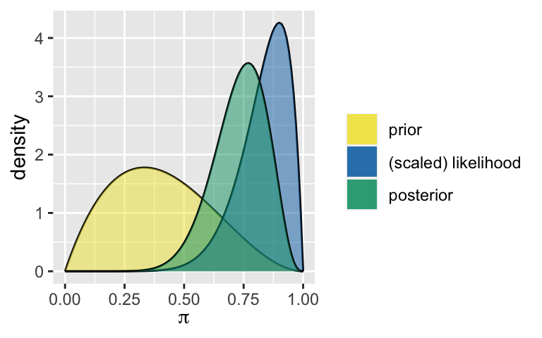
summarize_beta_binomial(alpha = 2, beta = 3, y = 9, n = 10)
##       model alpha beta      mean      mode        var        sd
## 1     prior     2    3 0.4000000 0.3333333 0.04000000 0.2000000
## 2 posterior    11    4 0.7333333 0.7692308 0.01222222 0.1105542
7.4 Solutions
- Bayesian estimation
\[\begin{split} E(\pi | Y = 150) & = \frac{151}{151 + 852} = 0.1505 \\ Mode(\pi | Y = 150) & = \frac{151 - 1}{151 + 852 - 2} = 0.1499 \\ \end{split}\]
- Bayesian interval estimation
Take the middle 95%:
qbeta(c(0.025, 0.975), 151, 852)
## [1] 0.1291000 0.1733164
There’s a 95% posterior probability that \(\pi\), the proportion of people that don’t believe in climate change, is between 0.129 and 0.173.
1 or 0. It is or it isn’t.
- Bayesian hypothesis testing
Plausible. The majority of the posterior falls above 0.13.
Plausible. The majority of the CI falls above 0.13.
There’s a high probability that this claim is correct.
1 - pbeta(0.13, shape1 = 151, shape2 = 852)
## [1] 0.9694835
\(P(\pi > 0.13 | \overline{y} = 0.15)\): Given our polling results, this is the probability that the claim is correct.
We have strong evidence that this claim is correct.
Check out the simulation
Everything looks good.mcmc_trace(climate_sim, pars = "pi")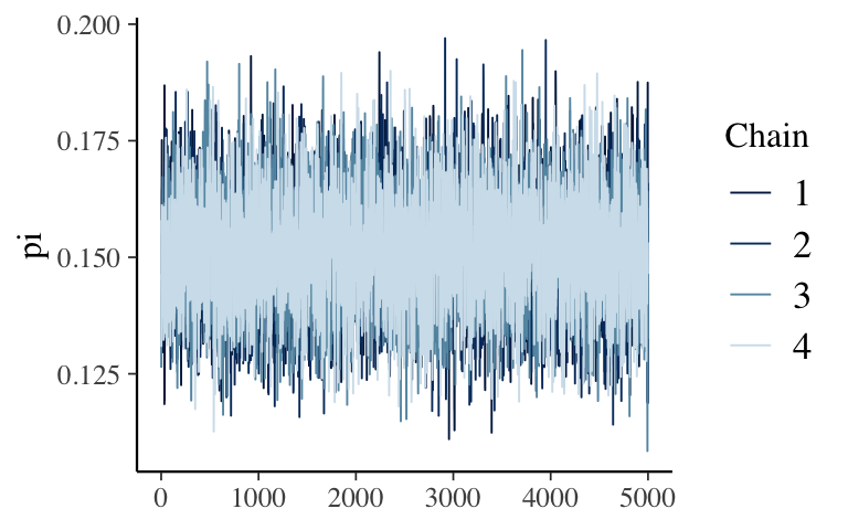
mcmc_dens_overlay(climate_sim, pars = "pi")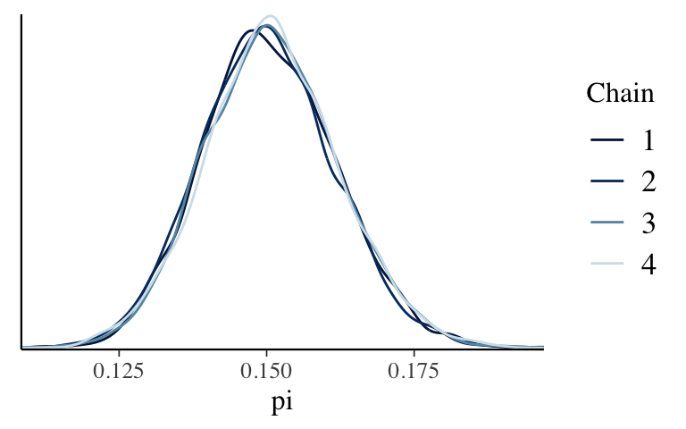
mcmc_dens(climate_sim, pars = "pi")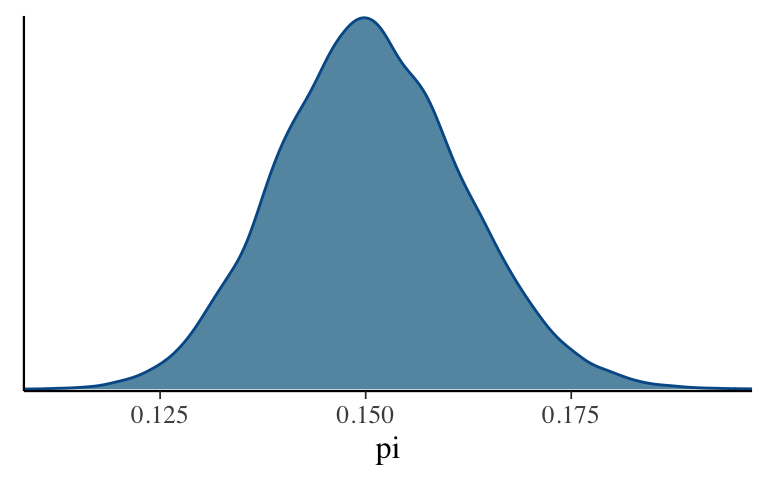
Prepare the simulation info
# Store the array of 4 chains in 1 data frame
climate_chains <- as.data.frame(
  climate_sim,
  pars = "lp__", include = FALSE)

# Check out the results
dim(climate_chains)
## [1] 20000     1
head(climate_chains)
##          pi
## 1 0.1551602
## 2 0.1466082
## 3 0.1471497
## 4 0.1508684
## 5 0.1641593
## 6 0.1651653
Simulate: Bayesian estimation
climate_chains %>%
  summarize(mean(pi), sample_mode(pi))
##    mean(pi) sample_mode(pi)
## 1 0.1506616       0.1497705
Simulate: Bayesian interval estimation
climate_chains %>%
  summarize(quantile(pi, 0.025), quantile(pi, 0.975))
##   quantile(pi, 0.025) quantile(pi, 0.975)
## 1           0.1291498           0.1736205
Simulate: Bayesian hypothesis testing
climate_chains %>%
  summarize(mean(pi > 0.13))
##   mean(pi > 0.13)
## 1          0.9701
MCMC shortcuts
# Calculate the posterior median & 95% CI
tidy(climate_sim, conf.int = TRUE, conf.level = 0.95)
## # A tibble: 1 x 5
##   term  estimate std.error conf.low conf.high
##   <chr>    <dbl>     <dbl>    <dbl>     <dbl>
## 1 pi       0.150    0.0113    0.129     0.174

# Plot the posterior & shade in the 95% CI
mcmc_areas(climate_sim, pars = "pi", prob = 0.95)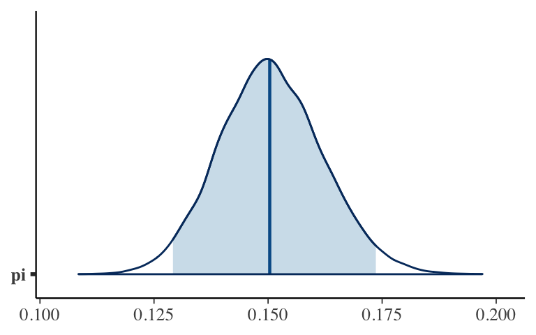
- Coding and communication drill
- Recommended: maximum likelihood
You will see something similar on homework.