19 Hierarchical modeling with multiple

GOALS

Dig deeper into a posterior analysis of a hierarchical model.

RECOMMENDED READING

Bayes Rules! Chapter 16.

19.1 Warm-up

In our Spotify analysis, let \(Y_{ij}\) denote the popularity of the \(i\)th song for artist \(j\). Then there are two equivalent ways to express our hierarchical “one-way ANOVA” model:

\[\begin{split} Y_{ij} | \mu_j, \sigma_y & \sim N(\mu_j, \sigma_y^2) \\ \mu_j | \mu, \sigma_\mu & \stackrel{ind}{\sim} N(\mu, \sigma_\mu^2) \\ \mu & \sim N(m, s^2) \\ \sigma_y & \sim \text{Exp}(l_y) \\ \sigma_\mu & \sim \text{Exp}(l_{\mu}) \\ \end{split}\]

where

• \(\mu_j\) = the typical song popularity for artist \(j\)
  
• \(\mu\) = the typical song popularity for the typical artist
• \(\sigma_y\) = the variability in popularity from song to song within any individual artist
• \(\sigma_\mu\) = the variability in typical popularity from artist to artist

Or, letting \(b_j = \mu_j - \mu\) denote a subject-specific tweak:

\[\begin{split} Y_{ij} | \mu_j, \sigma_y & \sim N(\mu_j, \sigma_y^2) \;\; \text{ with } \mu_j = \mu + b_j \\ b_j | \sigma_\mu & \stackrel{ind}{\sim} N(0, \sigma_\mu^2) \\ \mu & \sim N(m, s^2) \\ \sigma_y & \sim \text{Exp}(l_y) \\ \sigma_\mu & \sim \text{Exp}(l_{\mu}) \\ \end{split}\]

Then we can simulate the hierarchical posterior model:

# Load packages
library(bayesrules)
library(tidyverse)
library(rstanarm)
library(broom.mixed)
library(tidybayes)
library(forcats)
library(bayesplot)

# Load & reorder artist levels
data(spotify)
spotify <- spotify %>%
  select(artist, title, popularity) %>%
  mutate(artist = fct_reorder(artist, popularity, .fun = 'mean'))

# Calculate the mean popularity & number of songs for each artist
artist_means <- spotify %>%
  group_by(artist) %>%
  summarize(count = n(), popularity = mean(popularity))

# Simulate the posterior hierarchical model
hierarchical_model <- stan_glmer(
  popularity ~ (1 | artist), data = spotify,
  family = gaussian,
  chains = 4, iter = 5000*2, seed = 84735, refresh = 0)

WARM-UP 1: posterior predictions

In the previous activity we explored posterior predictions from this model. Consider two posterior predictive models.

1. Why does it make sense that Frank Ocean’s posterior predictive model higher than yours?
2. Why does it make sense that Frank Ocean’s posterior predictive model narrower than yours?

# Simulate the posterior predictive models
set.seed(84735)
two_predictions <- posterior_predict(
  hierarchical_model,
  newdata = data.frame(artist = c("you", "Frank Ocean")))

# Plot the posterior predictive models
mcmc_areas(two_predictions, prob = 0.8) +
  xlab("popularity") +
  ggplot2::scale_y_discrete(labels = c("you", "Frank Ocean"))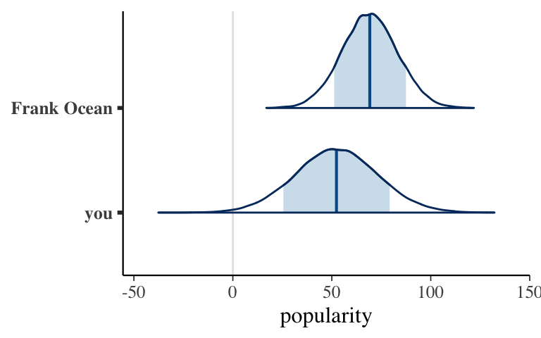

WARM-UP 2: shrinkage

Consider summaries of the posterior predictive models for all artists in our sample.

1. This plot displays the “shrinkage” phenomenon. What does this mean?

2. Why is Sean Kingston’s posterior median prediction shrunk more than Frank Ocean’s?

3. Why is Mia X’s posterior median prediction (at the lower end) shrunk more than Michael Kiwanuka’s?

# Simulate posterior predictive model of song popularity for each artist
set.seed(84735)
predictions_hierarchical <-  posterior_predict(
  hierarchical_model, newdata = artist_means)

# Plot posterior prediction intervals for each artist
ppc_intervals(
    artist_means$popularity,
    yrep = predictions_hierarchical,
    prob_outer = 0.80) +
    geom_hline(yintercept = 58.4, linetype = "dashed") +
  ggplot2::scale_x_continuous(
    labels = artist_means$artist,
    breaks = 1:nrow(artist_means)) +
    xaxis_text(angle = 90, hjust = 1)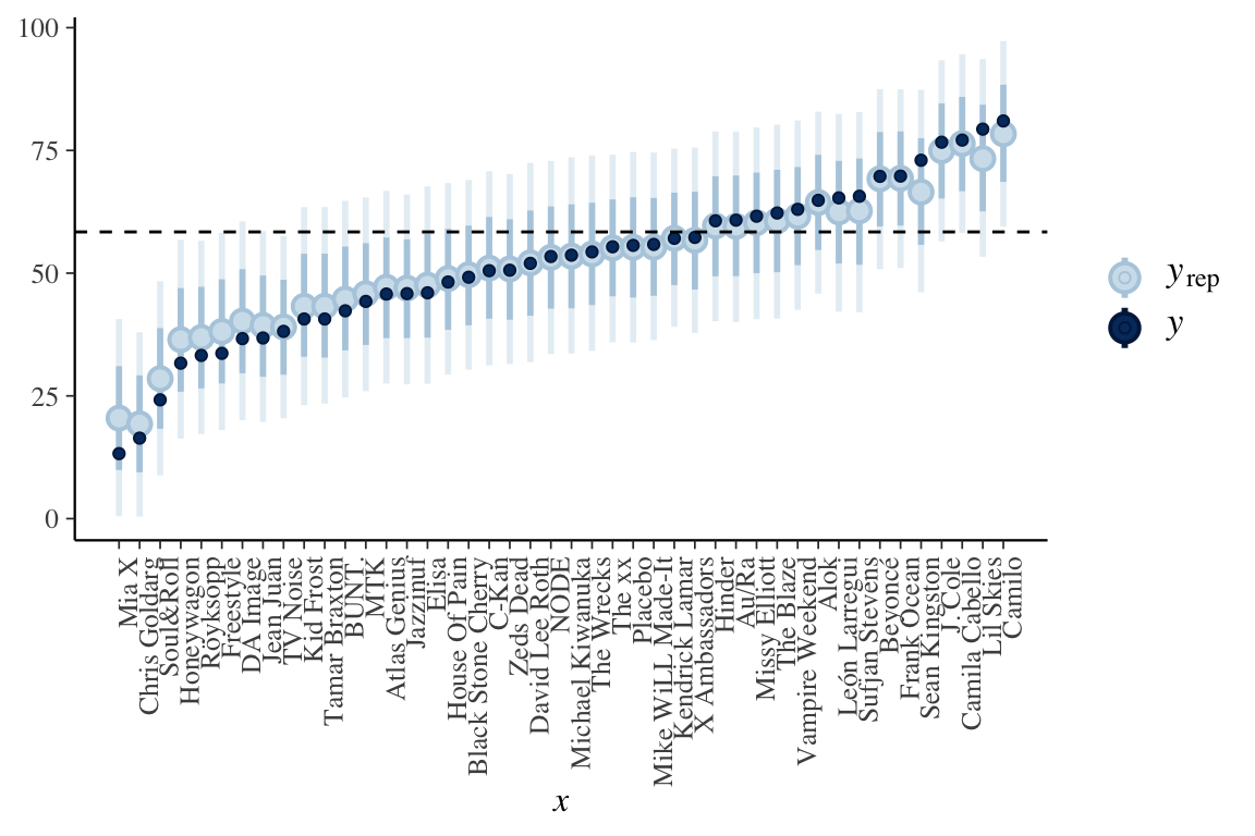

19.2 Exercises

Goals

Ask some follow-up posterior questions about our Spotify model.

1. Check in with your group
   What’s one thing you did for fun this past week?

2. Still matters: Prior specification
   In our simulation, we utilized weakly informative priors. Check out the prior specifications below and interpret the prior model on \(\mu\) (Intercept) in the context of the Spotify analysis. Note whether this is informative or not.

   prior_summary(hierarchical_model)

3. Still matters: MCMC diagnostics
   Our hierarchical posterior model was simulated using MCMC techniques. Construct 2 types of plots that help you assess whether this simulation has stabilized, hence whether we should trust the resulting posterior approximations.
   NOTE: There are 47 total parameters in our model: 44 \(\mu_j\) terms, \(\mu\), \(\sigma_\mu\), and \(\sigma_y\). Plotting the chain results for all of them would take some time. Instead, you might start by focusing on just the global parameters \(\mu\), \(\sigma_\mu\), and \(\sigma_y\) by including the following argument: pars = vars(-contains(" artist:")).

4. Still matters: pp_check (and other model evaluation questions)
   Before analyzing the posterior, it’s important to question how wrong our model might be. To this end, do a pp_check(). NOTE: Before applying this model, it would also be important to question its fairness and evaluate the quality of its posterior predictions, but we won’t do that here.

5. Posterior analysis: global mean \(\mu\)
   With some reassurance about our simulation and model, let’s dig into some posterior summaries. Let’s start with the global parameters that apply to all artists, not just those in our sample. To this end, we’ll first explore \(\mu\).
   • Take note of the syntax!
     
   • Interpret the 80% posterior credible interval for \(\mu\) ((Intercept)) in the context of the Spotify analysis.

   tidy(hierarchical_model, effects = "fixed",
        conf.int = TRUE, conf.level = 0.80)

6. Posterior analysis: global standard deviation parameters \(\sigma_\mu\) and \(\sigma_y\)
   Next, consider the global standard deviation parameters. Take note of the syntax!

   tidy(hierarchical_model, effects = "ran_pars")

   1. How can we interpret the posterior median estimate of \(\sigma_\mu\), sd_(Intercept).artist?
      • Across all songs and artists, the typical song popularity varies with standard deviation 15.2.
        
      • The typical song popularity varies by 15.2 points from artist to artist.
      • Song popularity varies by 15.2 points from song to song within individual artists.
   2. How can we interpret the posterior median estimate of \(\sigma_y\), sd_Observation.Residual?
      • Across all songs and artists, the typical song popularity varies with standard deviation 14.0.
        
      • The typical song popularity varies by 14.0 points from artist to artist.
      • Song popularity varies by 14.0 points from song to song within individual artists.

7. Decomposition of variance
   One powerful aspect of hierarchical models is that they help us better understand the variability in song popularity. Specifically, we can decompose the total variability in popularity across all songs and artists by the variability due to differences in artists (\(\sigma_\mu^2\)) and the variability in songs within artists (\(\sigma_y^2\)):

   \[Var(Y) = \sigma_\mu^2 + \sigma_y^2\]

   1. Using the spotify data, calculate the observed total variability in popularity across all songs and artists.
   2. Prove that this total variability is equal to the sum of the observed \(\sigma_\mu^2\) (15.2^2) and \(\sigma_y^2\) (14.0^2). NOTE: The results will be off due to rounding.

8. Analysis of variance
   In light of the previous exercise:
   1. What proportion of the variability in popularity from song to song is due to differences between artists? NOTE: For consistency, just use the 15.2 and 14.0 numbers in your calculation, not the total variability calculated from scratch.
      
   2. What proportion of the variability in popularity from song to song is due to fluctuations in song popularity within individual artists?

9. Posterior analysis: groups (part 1)
   Now that we have a sense of the global parameters, hence the population of all artists, let’s consider the group-specific patterns among our sampled artists. First, obtain the posterior summaries for the “tweak” parameters \(b_j\).

   • Take note of the syntax.
   • Interpret the posterior median estimates for Mia_X and Camilo.

   artist_summary <- tidy(
     hierarchical_model, effects = "ran_vals",
     conf.int = TRUE, conf.level = 0.80)
   
   # Check it out
   artist_summary

10. Posterior analysis: groups (part 2)
    In some cases, we might wish to convert our observations about \(b_j\) to observations about the group-specific means \(\mu_j\):

    \[\mu_j = \mu + b_j\]

    This is possible, but the syntax is messy. Check out each chunk below one at a time and note what’s going on:

    # Get MCMC chains for each mu_j (using tidybayes)
    artist_chains <- hierarchical_model %>%
      spread_draws(`(Intercept)`, b[,artist]) %>%
      mutate(mu_j = `(Intercept)` + b)
    
    # Check it out
    artist_chains %>%
      select(artist, `(Intercept)`, b, mu_j) %>%
      head()

    # Get posterior summaries for mu_j
    artist_summary_scaled <- artist_chains %>%
      select(-`(Intercept)`, -b) %>%
      mean_qi(.width = 0.80) %>%
      mutate(artist = fct_reorder(artist, mu_j))
    
    # Check it out
    artist_summary_scaled %>%
      select(artist, mu_j, .lower, .upper) %>%
      head()

    # Plot the posterior models of mu_j for all artists
    ggplot(
        artist_summary_scaled,
        aes(x = artist, y = mu_j, ymin = .lower, ymax = .upper)) +
        geom_pointrange() +
        xaxis_text(angle = 90, hjust = 1)

11. Posterior analysis: groups (part 3)
    Consider some follow-up questions for the previous exercise.
    1. Why are the posterior models of \(\mu_j\) much narrower than the posterior predictive models for the artists that we reviewed in the warm-up?
       
    2. Why is the posterior model for Sean Kingston’s \(\mu_j\) term much wider than that for Frank Ocean’s?

12. Posterior prediction (part 1)
    Finally, let’s do some posterior prediction. You’ve already used the shortcut posterior_predict() function, but it’s important to understand how these predictions are made. To do this from scratch, we can use the 20,000 MCMC values for each parameter. Run the chunk below and check out how these chains are labeled:

    • \(\mu\) = (Intercept)
    • \(b_j\) = [(Intercept) artist:j]
    • \(\sigma_y\) = sigma
      NOTE: this is on the standard deviation scale
    • \(\sigma_\mu^2\) = Sigma[artist:(Intercept),(Intercept)]
      NOTE: this is on the variance scale

    # Store the simulation in a data frame
    hierarchical_model_df <- as.data.frame(hierarchical_model)
    
    # Check out the first 3 and last 3 parameter labels
    hierarchical_model_df %>%
      colnames() %>%
      as.data.frame() %>%
      slice(1:3, 45:47)

13. Posterior prediction (part 2)
    Let’s start by predicting the popularity of the next song for an artist in our sample: Frank_Ocean. Since we observed Ocean, we have a posterior understanding of their tweak \(b_j\), hence mean popularity \(\mu_j\). Thus we only need to appeal to the fact that:

    \[Y | \mu_j, \sigma_y \sim N(\mu_j, \sigma_y^2)\]

    Simulate and plot the posterior predictive model for Ocean’s next song. Some starting code is provided.

    ocean_chains <- hierarchical_model_df %>%
      mutate(b = `b[(Intercept) artist:Frank_Ocean]`,
             sigma_y = sigma) %>%
      select(`(Intercept)`, b, sigma_y)
    
    # Check it out
    head(ocean_chains)

14. Posterior prediction (part 3)
    Next, let’s predict the popularity of your next song on Spotify. Since we didn’t observe any data on you, we don’t have any posterior understanding of your mean popularity \(\mu_j\). Thus we must appeal to the fact that:

    \[\begin{split} Y | \mu_j, \sigma_y & \sim N(\mu_j, \sigma_y^2) \\ \mu_j | \mu, \sigma_\mu & \sim N(\mu, \sigma_\mu^2) \\ \end{split}\]

    Simulate and plot the posterior predictive model for your next song. Some starting code is provided.

    your_chains <- hierarchical_model_df %>%
      mutate(sigma_y = sigma,
             sigma_mu = sqrt(`Sigma[artist:(Intercept),(Intercept)]`)) %>%
      select(`(Intercept)`, sigma_mu, sigma_y)
    
    # Check it out
    head(your_chains)

15. Posterior prediction follow-up
    Re-examine the plots of the posterior predictive models for you and Frank Ocean. Now better understanding how these models are simulated, explain mathematically (not just intuitively) why your model is wider than Ocean’s.

19.3 Solutions

1. Check in with your group

2. Still matters: Prior specification
   \(\mu \sim N(58, 52^2)\)
   We understand that the average song popularity (across all songs and artists) is around 58, though are very uncertain. It’s plausible that \(\mu\) falls anywhere between -46 and 162 (\(58 \pm 2*52\)). This is outside the range of actual popularity levels, 0 – 100.

   prior_summary(hierarchical_model)
   ## Priors for model 'hierarchical_model' 
   ## ------
   ## Intercept (after predictors centered)
   ##   Specified prior:
   ##     ~ normal(location = 58, scale = 2.5)
   ##   Adjusted prior:
   ##     ~ normal(location = 58, scale = 52)
   ## 
   ## Auxiliary (sigma)
   ##   Specified prior:
   ##     ~ exponential(rate = 1)
   ##   Adjusted prior:
   ##     ~ exponential(rate = 0.048)
   ## 
   ## Covariance
   ##  ~ decov(reg. = 1, conc. = 1, shape = 1, scale = 1)
   ## ------
   ## See help('prior_summary.stanreg') for more details

3. Still matters: MCMC diagnostics
   Looks stable.

   mcmc_trace(hierarchical_model, pars = vars(-contains(" artist:")))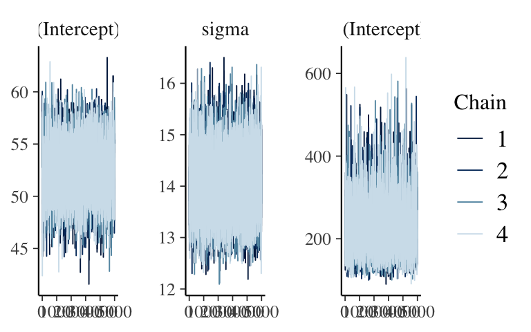

   

   mcmc_dens_overlay(hierarchical_model, pars = vars(-contains(" artist:")))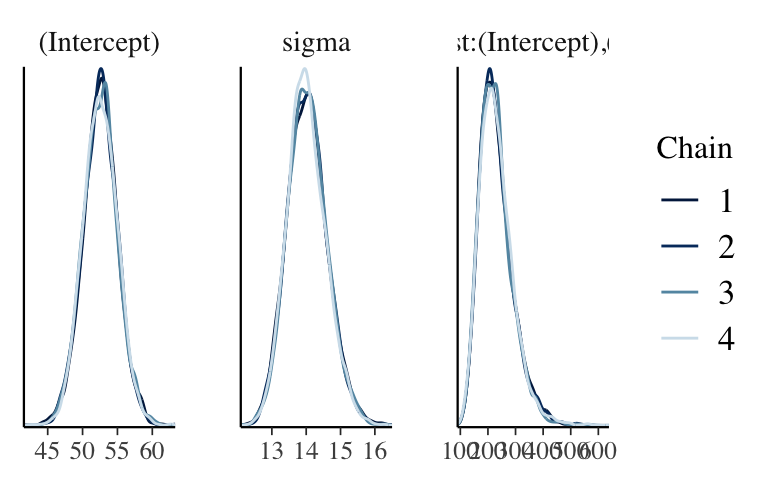

   

4. Still matters: pp_check (and other model evaluation questions)
   Looks pretty good.

   pp_check(hierarchical_model)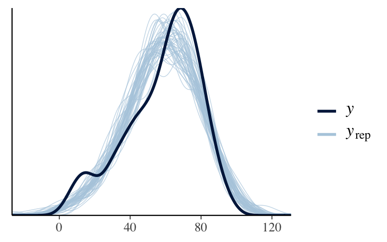

   

5. Posterior analysis: global mean \(\mu\)
   There’s an 80% chance that the average song popularity is somewhere between 49.3 and 55.6.

   tidy(hierarchical_model, effects = "fixed",
        conf.int = TRUE, conf.level = 0.80)
   ## # A tibble: 1 x 5
   ##   term        estimate std.error conf.low conf.high
   ##   <chr>          <dbl>     <dbl>    <dbl>     <dbl>
   ## 1 (Intercept)     52.5      2.42     49.3      55.6

6. Posterior analysis: global standard deviation parameters \(\sigma_\mu\) and \(\sigma_y\)

   tidy(hierarchical_model, effects = "ran_pars")
   ## # A tibble: 2 x 3
   ##   term                    group    estimate
   ##   <chr>                   <chr>       <dbl>
   ## 1 sd_(Intercept).artist   artist       15.2
   ## 2 sd_Observation.Residual Residual     14.0

   1. The typical song popularity varies by 15.2 points from artist to artist.
      
   2. Song popularity varies by 14.0 points from song to song within individual artists.

7. Decomposition of variance

   spotify %>%
     summarize(var(popularity))
   ## # A tibble: 1 x 1
   ##   `var(popularity)`
   ##               <dbl>
   ## 1              426.
   
   15.2^2 + 14.0^2
   ## [1] 427.04

8. Analysis of variance

   # a: roughly 54%
   15.2^2 / (15.2^2 + 14.0^2)
   ## [1] 0.5410266
   
   # b: roughly 46%
   14.0^2 / (15.2^2 + 14.0^2)
   ## [1] 0.4589734

9. Posterior analysis: groups (part 1)
   Our posterior median guess is that Mia X’s typical song popularity is 32.1 points below that of the typical artist and that Camilo’s is 25.9 points above that of a typical artist.

   artist_summary <- tidy(
     hierarchical_model, effects = "ran_vals",
     conf.int = TRUE, conf.level = 0.80)
   artist_summary %>%
     filter(level %in% c("Mia_X", "Camilo"))
   ## # A tibble: 2 x 7
   ##   level  group  term        estimate std.error conf.low conf.high
   ##   <chr>  <chr>  <chr>          <dbl>     <dbl>    <dbl>     <dbl>
   ## 1 Mia_X  artist (Intercept)    -32.1      6.85    -40.9     -23.2
   ## 2 Camilo artist (Intercept)     25.9      5.04     19.5      32.4

10. Posterior analysis: groups (part 2)

    # Get MCMC chains for each mu_j (using tidybayes)
    artist_chains <- hierarchical_model %>%
      spread_draws(`(Intercept)`, b[,artist]) %>%
      mutate(mu_j = `(Intercept)` + b)
    
    # Check it out
    artist_chains %>%
      select(artist, `(Intercept)`, b, mu_j) %>%
      head()
    ## # A tibble: 6 x 4
    ## # Groups:   artist [6]
    ##   artist                    `(Intercept)`      b  mu_j
    ##   <chr>                             <dbl>  <dbl> <dbl>
    ## 1 artist:Alok                        49.6   8.67  58.2
    ## 2 artist:Atlas_Genius                49.6 -11.8   37.8
    ## 3 artist:Au/Ra                       49.6   6.91  56.5
    ## 4 artist:Beyoncé                     49.6  21.7   71.3
    ## 5 artist:Black_Stone_Cherry          49.6  -1.63  48.0
    ## 6 artist:BUNT.                       49.6  -3.80  45.8
    
    # Get posterior summaries for mu_j
    artist_summary_scaled <- artist_chains %>%
      select(-`(Intercept)`, -b) %>%
      mean_qi(.width = 0.80) %>%
      mutate(artist = fct_reorder(artist, mu_j))
    
    # Check it out
    artist_summary_scaled %>%
      select(artist, mu_j, .lower, .upper) %>%
      head()
    ## # A tibble: 6 x 4
    ##   artist                     mu_j .lower .upper
    ##   <fct>                     <dbl>  <dbl>  <dbl>
    ## 1 artist:Alok                64.3   60.2   68.3
    ## 2 artist:Atlas_Genius        47.0   38.9   55.3
    ## 3 artist:Au/Ra               59.5   52.2   66.9
    ## 4 artist:Beyoncé             69.1   65.6   72.6
    ## 5 artist:Black_Stone_Cherry  49.7   42.7   56.6
    ## 6 artist:BUNT.               44.6   35.6   53.6
    
    # Plot the posterior models of mu_j for all artists
    ggplot(
        artist_summary_scaled,
        aes(x = artist, y = mu_j, ymin = .lower, ymax = .upper)) +
        geom_pointrange() +
        xaxis_text(angle = 90, hjust = 1)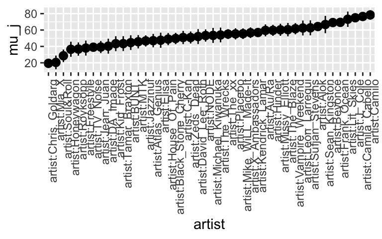

    

11. Posterior analysis: groups (part 3)
    1. It’s easier to predict averages than individual outcomes
       
    2. Kingston has a smaller sample size:

    artist_means %>%
      filter(artist %in% c("Frank Ocean", "Sean Kingston"))
    ## # A tibble: 2 x 3
    ##   artist        count popularity
    ##   <fct>         <int>      <dbl>
    ## 1 Frank Ocean      40       69.8
    ## 2 Sean Kingston     2       73

12. Posterior prediction (part 1)

    # Store the simulation in a data frame
    hierarchical_model_df <- as.data.frame(hierarchical_model)
    
    # Check out the first 3 and last 3 parameter labels
    hierarchical_model_df %>%
      colnames() %>%
      as.data.frame() %>%
      slice(1:3, 45:47)
    ##                                       .
    ## 1                           (Intercept)
    ## 2           b[(Intercept) artist:Mia_X]
    ## 3   b[(Intercept) artist:Chris_Goldarg]
    ## 4          b[(Intercept) artist:Camilo]
    ## 5                                 sigma
    ## 6 Sigma[artist:(Intercept),(Intercept)]

13. Posterior prediction (part 2)

    ocean_chains <- hierarchical_model_df %>%
      mutate(b = `b[(Intercept) artist:Frank_Ocean]`,
             sigma_y = sigma) %>%
      select(`(Intercept)`, b, sigma_y)
    
    # Check it out
    head(ocean_chains)
    ##   (Intercept)        b  sigma_y
    ## 1    49.57965 18.84581 14.03869
    ## 2    50.29540 20.63330 13.24216
    ## 3    49.24916 19.09251 14.27937
    ## 4    51.51161 16.17393 14.28986
    ## 5    50.55764 20.18176 13.35980
    ## 6    50.77513 20.51210 14.79863
    
    ocean_chains %>%
      mutate(y = rnorm(20000, mean = `(Intercept)` + b, sd = sigma_y)) %>%
      ggplot(., aes(x = y)) +
        geom_density()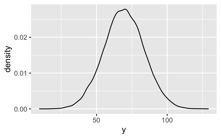

    

14. Posterior prediction (part 3)

    your_chains <- hierarchical_model_df %>%
      mutate(sigma_y = sigma,
             sigma_mu = sqrt(`Sigma[artist:(Intercept),(Intercept)]`)) %>%
      select(`(Intercept)`, sigma_mu, sigma_y)
    
    # Check it out
    head(your_chains)
    ##   (Intercept) sigma_mu  sigma_y
    ## 1    49.57965 14.21865 14.03869
    ## 2    50.29540 14.48935 13.24216
    ## 3    49.24916 13.54214 14.27937
    ## 4    51.51161 12.74468 14.28986
    ## 5    50.55764 13.13252 13.35980
    ## 6    50.77513 12.46346 14.79863
    
    your_chains %>%
      mutate(mu_you = rnorm(20000, mean = `(Intercept)`, sd = sigma_mu)) %>%
      mutate(y = rnorm(20000, mean = mu_you, sd = sigma_y)) %>%
      ggplot(., aes(x = y)) +
        geom_density()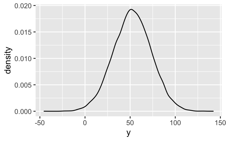

    

15. Posterior prediction follow-up
    It incorporates an additional source of variability: between artists.