3 The Beta-Binomial model
GOAL
Explore a fundamental Bayesian model: the Beta-Binomial.
RECOMMENDED READING
Bayes Rules! Chapter 3.
HEADS UP
We’ll be using some new Greek letters today: \(\pi\) = “pi,” \(\alpha\) = “alpha,” \(\beta\) = “beta”
3.1 Warm-up
WARM-UP 1
As a first step in any Bayesian analysis, we must tune a prior model for our parameter of interest. Sketch a prior pdf \(f(\pi)\) for each of the following proportions \(\pi\). Include labels to indicate which prior is which!
- \(\pi_1\) = the current U.S. unemployment rate
- \(\pi_2\) = Biden’s current approval rating
- \(\pi_3\) = proportion of Mac students that have the sinistromanualauriculares condition (looking up this term is off limits for this exercise!)
WARM-UP 2
Consider \(\pi_3\), the proportion of Mac students that have the sinistromanualauriculares condition. Suppose that in a survey of \(n = 100\) students, \(Y = 70\) have this condition. Below, sketch your prior pdf of \(\pi_3\) from the previous exercise along with an updated posterior pdf, \(f(\pi_3|y = 70)\), in light of this data.

BETA-BINOMIAL FRAMEWORK
The Beta-Binomial model can inform our understanding of \(\pi\) within the following framework:
parameter of interest: \(\pi\)
proportion \(\pi\) is a continuous random variable:
\[\pi \in [0,1]\] For example, \(\pi\) might be a politician’s approval rating, U.S. unemployment rate, a player’s batting average, etc. The Beta probability model, which also lives on \([0,1]\), is a natural choice for the prior.data: \(Y\)
\(Y\) is the number of successes in \(n\) independent trials where the probability of success in each trial is \(\pi\). The dependence of \(Y\) on \(\pi\) can therefore be described by a Binomial model.
BETA WARM-UP
Suppose \(\pi\) has pdf \(f(\pi) \propto \pi^{4} (1-\pi)^{3}\) for \(\pi \in [0,1]\).

- Specify the model of \(\pi\).
- Specify the missing normalizing constant for \(f(\pi)\).
- Calculate \(\int_0^1 \pi^{4} (1-\pi)^{3} d\pi\).
3.2 Exercises
You’re running for MCSG class president! Let \(\pi\) be your level of support, ie. the proportion of students that plan to vote for you.
Prior: \(f(\pi)\)
Before taking any formal polls, your campaign manager defines the following prior model for \(\pi\) based on some small market research:
\[\pi \sim Beta(1,4)\]Write out the formula for prior pdf \(f(\pi)\). Further, take a personal note of your manager’s prior: what range of election support \(\pi\) do they find plausible?

- Data model: \(f(y | \pi)\)
To learn about \(\pi\), your manager polls 10 students. Let \(Y\) be the number that support you.- Specify the conditional model which captures the dependence of \(Y\) on \(\pi\), \(Y | \pi \sim ???\).
- Write out a formula for the conditional pmf \(f(y|\pi)\).
- The conditional pmf is plotted below for a range of just 3 plausible \(\pi\) values along the [0,1] continuum: (0.2, 0.5, 0.8). Describe the punchlines – how does \(Y\) depend upon \(\pi\)?

The data are in! \(L(\pi|y = 6)\)
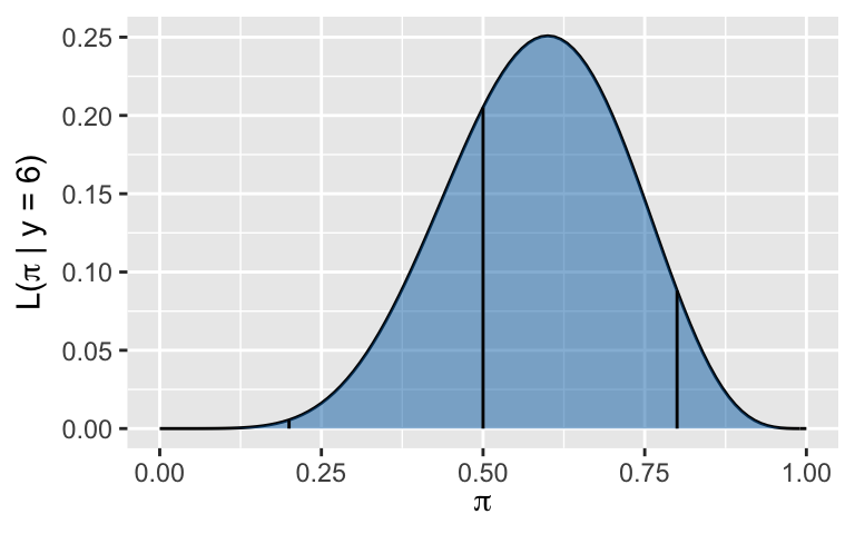
In this first poll, \(Y = 6\) of the 10 polled students support you. Exciting!- Write out a formula for the likelihood function, \(L(\pi|y = 6)\).
- \(L(\pi|y=6)\) is plotted below for all \(\pi \in [0,1]\). For context, the vertical lines represent the likelihood evaluated at the 3 values of \(\pi\) considered in the previous exercise. Recall that \(L(\pi|y=6)\) is a function (but NOT a pdf) of your unknown election support \(\pi\). It allows us to assess the compatibility of our known data (\(Y = 6\) of the 10 students support you) with \(\pi\) values on the range between 0 and 1. Based on this likelihood function, with what levels of support \(\pi\) are the observed poll results most compatible?
- Normalizing constant \(f(y = 6)\)
We’ve now evaluated the compatibility of the poll result with various levels of election support \(\pi\). For frame of reference, calculate the normalizing constant \(f(y=6)\), i.e. the overall chance of observing \(Y = 6\) across all possible \(\pi\). NOTE:- Your answer should be a constant which doesn’t depend upon \(\pi\) or “\(y\).”
- Don’t take time to simplify the \(\Gamma(\cdot)\) terms. Many pieces will cancel out in later exercises.
- Construct the posterior: \(f(\pi | y = 6)\)
The plot below illustrates the manager’s prior \(f(\pi)\) and a scaled version of the likelihood function corresponding to the polling data \(Y = 6\), \(L(\pi | y = 6)\). Before doing any formal calculations, sketch what you anticipate their posterior model of \(\pi\) will look like.

Construct the posterior pdf of \(\pi\), \(f(\pi | y=6)\). No need to define any normalizing constants.
Use the posterior pdf to specify the posterior model of \(\pi\) given \(Y = 6\): \[\pi|(Y=6) \sim ???\]
Interpret the posterior
The posterior pdf is plotted below. Describe your manager’s posterior understanding about your election support \(\pi\) and how this compares to their prior understanding.
- Utilizing proportionality
In the previous exercises, you constructed the posterior pdf using Bayes’ Rule: \[f(\pi|y=6) = \frac{f(\pi)L(\pi|y=6)}{f(y=6)}\] You did more work than necessary! Since \(f(y=6)\) doesn’t depend upon \(\pi\), it’s merely a normalizing constant for the posterior pdf. That is, \[f(\pi|y=6) = c f(\pi)L(\pi|y=6) \propto f(\pi)L(\pi|y=6)\] With this in mind, construct \(f(\pi|y=6)\) from \(L(\pi|y=6)\) and \(f(\pi)\) alone. HINT: Keep dropping constants from your formula until the only pieces remaining depend upon \(\pi\).
Alternative reality
What if, instead, we had observed that 9 in 10 polled students support you? Starting from the original Beta(1,4) prior, construct the posterior model of \(\pi\) in this alternative reality (plotted below) and compare this with the posterior based on the 6-out-of-10 poll.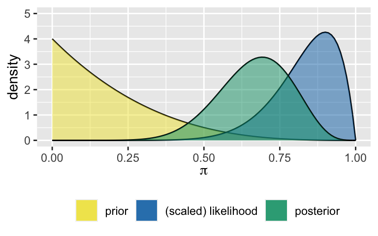
Building the general Beta-Binomial model
In general, let \(\pi \in [0,1]\) be a proportion about which we express our prior information by \(\pi \sim Beta(\alpha, \beta)\). To make inferences about \(\pi\), we conduct \(n\) independent trials, each with probability of success \(\pi\), and observe the number of successes \(Y\), thus \(Y|\pi \sim Bin(n,\pi)\). Specify the posterior model of \(\pi\) upon observing data \(Y = y\):\[\begin{split} Y|\pi & \sim Bin(n,\pi) \\ \pi & \sim Beta(\alpha, \beta) \\ \end{split} \Rightarrow \pi|(Y=y) \sim ???\]
- Conjugate prior
The Beta prior of the Beta-Binomial model is called a conjugate prior since it produces a posterior from the same Beta “family,” just differently tuned. Reexamine the prior pdf and likelihood function and explain why we might anticipate that their combination would produce this conjugacy.
A conjugate prior is one that produces a posterior model in the same “family.” For example, both the prior and posterior in the Beta-Binomial are from the Beta family. Conjugate priors make the math easier!
Tuning the Beta prior
We started our analysis with a pre-tuned prior model. In some cases, we’ll need to do this on our own. Use the shiny apps below to interact with the Beta pdf and explore how we might tune the Beta model to reflect our prior understanding of \(\pi\). Specifically, identify combinations of \(\alpha\) and \(\beta\) that reflect the following priors. There are many reasonable answers!- We’re pretty certain that \(\pi\) is near 0.
- We’re very certain that \(\pi\) is near 0.5.
- We’re vaguely certain that \(\pi\) is near 0.5.
- We have no idea – \(\pi\) is equally likely to be anywhere between 0 and 1.
NOTE: If you don’t want to play around with shiny, you can utilize the
plot_beta()andsummarize_beta()functions from the bayesrules package:plot_beta(alpha = ___, beta = ___) summarize_beta(alpha = ___, beta = ___)
3.3 Shiny apps
You’ll be building your own shiny apps in homework and they’ll be handy for your capstone project. Below is some code for bare bones shiny apps. To see what else is possible, check out these examples! If you are new to shiny, play around with the code, identify what each line accomplishes, and experiment by making some small changes. If you’re not new to shiny, try to make these apps more aesthetically pleasing!
Getting started
If it’s not already, install the shiny package by typing the following in the console (NOT Rmd):
install.packages("shiny")Then load the library:
library(shiny)
library(bayesrules)  # for the plotting functions
As you work through the exercises below, note that shiny apps consist of 2 pieces:
server
Instructions for building the app - what plot to make, what quantities to calculate, etc.ui (user interface)
Controls the layout, appearance, and widgets (eg: slide bars). This is where you can make this aesthetically pleasing (in contrast to our simple apps above).
Shiny app 1: a simple interactive Beta pdf
# Build the server
server1 <- function(input, output) {
  output$priorPdf <- renderPlot({
    plot_beta(alpha = input$aPrior, beta = input$bPrior) +
      lims(y=c(0,input$ymax))
  })
}

# Build the user interface
ui1 <- fluidPage(
  sidebarLayout(
    sidebarPanel(
      h4("Tune the Beta(alpha, beta) prior:"),
      sliderInput("aPrior", "alpha", min = 0, max = 100, value = 1),
      sliderInput("bPrior", "beta", min = 0, max = 100, value = 1),
      h4("Specify the limit of the y-axis:"),
      sliderInput("ymax", "", min = 1, max = 40, value = 10)
    ),
    mainPanel(
      h4("Plot of the prior pdf:"),
      plotOutput("priorPdf")
    )
  )
)

# Run the shiny app!
shinyApp(ui = ui1, server = server1)
Shiny app 2: include more stuff
# Build the server
server2 <- function(input, output) {
  output$priorPdf <- renderPlot({
    plot_beta(alpha = input$aPrior, beta = input$bPrior) +
      lims(y = c(0, input$ymax))
  })

  output$priorTable <- renderTable({
    summarize_beta(alpha = input$aPrior, beta = input$bPrior)
  })
}


# Build the user interface
ui2 <- fluidPage(
  sidebarLayout(
    sidebarPanel(
      h4("Tune the Beta(a,b) prior:"),
      sliderInput("aPrior", "alpha", min = 0, max = 100, value = 1),
      sliderInput("bPrior", "beta", min = 0, max = 100, value = 1),
      h4("Specify the limit of the y-axis:"),
      sliderInput("ymax", "", min = 1, max = 40, value = 10)
    ),
    mainPanel(
      h4("Plot of the prior pdf:"),
      plotOutput("priorPdf"),
      h4("Prior features:"),
      tableOutput("priorTable")
    )
  )
)

# Run the shiny app!
shinyApp(ui = ui2, server = server2)
3.4 Solutions
- For \(\pi \in [0,1]\), \[f(\pi) = \frac{\Gamma(5)}{\Gamma(1)\Gamma(4)}\pi^{1-1}(1-\pi)^{4-1} = \frac{\Gamma(5)}{\Gamma(1)\Gamma(4)}(1-\pi)^{3}\]
- .
- \(Y|\pi \sim Bin(10, \pi)\)
- \(f(y|\pi) = \left(\begin{array}{c} 10 \\ y \end{array}\right) \pi^y (1-\pi)^{10-y}\) for \(y \in \{0,1,...,10\}\)
- The greater your election support \(\pi\), the greater the typical number of polled students that support you.
- .
- \(L(\pi|y=6) = \left(\begin{array}{c} 10 \\ 6 \end{array}\right) \pi^6 (1-\pi)^4\) for \(\pi \in [0,1]\)
- We most likely to have observed this poll result if your underlying election support is around 0.6. We’re unlikely to have observed this poll if your support is as low as, say, 0.3, or as high as, say 0.9.
- Since \(\pi\) is continuous, we need to integrate \(f(y=6,\pi)\) across all possible \(\pi\): \[\begin{split} f(y = 6) & = \int_0^1 f(y=6,\pi)d\pi \\ & = \int_0^1 f(y=6|\pi)f(\pi) d\pi \\ & = \int_0^1 \left(\begin{array}{c} 10 \\ 6 \end{array}\right) \pi^6 (1-\pi)^{10-6} \cdot \frac{\Gamma(5)}{\Gamma(1)\Gamma(4)}(1-\pi)^{3} d\pi \\ & = \left(\begin{array}{c} 10 \\ 6 \end{array}\right) \frac{\Gamma(5)}{\Gamma(1)\Gamma(4)} \int_0^1 \pi^6 (1-\pi)^7 d\pi \;\; \text{(take the constants out of the integral)} \\ & = \left(\begin{array}{c} 10 \\ 6 \end{array}\right) \frac{\Gamma(5)}{\Gamma(1)\Gamma(4)} \frac{\Gamma(7)\Gamma(8)}{\Gamma(15)} \int_0^1 \frac{\Gamma(15)}{\Gamma(7)\Gamma(8)} \pi^{7-1} (1-\pi)^{8-1} d\pi \;\; \text{(make the integrand look like a Beta pdf)}\\ & = \left(\begin{array}{c} 10 \\ 6 \end{array}\right) \frac{\Gamma(5)}{\Gamma(1)\Gamma(4)}\frac{\Gamma(7)\Gamma(8)}{\Gamma(15)} \;\; \text{(the Beta pdf integrates to 1)}\\\\ \end{split}\]
- .
- sketch
- \[\begin{split}
f(\pi | y=6)
& = \frac{f(\pi) L(\pi|y=6)}{f(y=6)} \\
& = \frac{\frac{\Gamma(5)}{\Gamma(1)\Gamma(4)} (1-\pi)^{3} \cdot \left(\begin{array}{c} 10 \\ 6 \end{array}\right) \pi^6 (1-\pi)^{4}}{ \left(\begin{array}{c} 10 \\ 6 \end{array}\right) \frac{\Gamma(5)}{\Gamma(1)\Gamma(4)} \frac{\Gamma(7)\Gamma(8)}{\Gamma(15)}} \\
& = \frac{\Gamma(15)}{\Gamma(7)\Gamma(8)} \pi^{7-1} (1-\pi)^{8-1} \\
\end{split}\]
- \(\pi | (Y=6) \sim Beta(7,8)\)
- .
- . \[\begin{split} f(\pi | y=6) & \propto f(\pi) L(\pi|y=6) \\ & = \frac{\Gamma(5)}{\Gamma(1)\Gamma(4)} (1-\pi)^{3} \cdot \left(\begin{array}{c} 10 \\ 6 \end{array}\right) \pi^6 (1-\pi)^{4} \\ & \propto (1-\pi)^{3} \cdot \pi^6 (1-\pi)^{4} \\ & = \pi^{7-1} (1-\pi)^{8-1} \\ \end{split}\]
- \(\pi|(Y=9) \sim Beta(10,5)\)
.
\[\pi|(Y=y) \sim Beta(\alpha+y, \beta+n-y)\]Proof:
\[\begin{split} f(\pi) & = \frac{\Gamma(\alpha + \beta)}{\Gamma(\alpha)\Gamma(\beta)} \pi^{\alpha - 1}(1-\pi)^{\beta - 1} \;\; \text{ for } \pi \in [0,1] \\ L(\pi|y) & = \left(\begin{array}{c} n \\ y \end{array} \right)\pi^y(1-\pi)^{n-y} \;\; \text{ for } \pi \in [0,1] \\ f(\pi|y) & \propto f(\pi)L(\pi|y) \\ & = \frac{\Gamma(\alpha + \beta)}{\Gamma(\alpha)\Gamma(\beta)} \pi^{\alpha - 1}(1-\pi)^{\beta - 1} \left(\begin{array}{c} n \\ y \end{array} \right)\pi^y(1-\pi)^{n-y} \\ & \propto \pi^{\alpha - 1}(1-\pi)^{\beta - 1} \pi^y(1-\pi)^{n-y} \\ & = \pi^{\alpha + y - 1}(1-\pi)^{\beta + n - y - 1} \\ \end{split}\]