15 Naive Bayes classification

GOALS

The overarching goal of the past few weeks has been to model some response variable $Y$ by predictors $X$:

When $Y$ is quantitative and bell-shaped (whether continuous or discrete), we might utilize a Normal regression model which assumes that
\[Y_i | \beta_0, \beta_1, \sigma \stackrel{ind}{\sim} N(\mu_i, \sigma^2) \;\; \text{ where } \mu_i = \beta_0 + \beta_1 X_i\]
When $Y$ is a quantitative count, we might utilize a Poisson (or Negative Binomial) regression model which assumes that
\[Y_i | \beta_0, \beta_1 \stackrel{ind}{\sim} Pois(\lambda_i) \;\; \text{ where } \log(\lambda_i) = \beta_0 + \beta_1 X_i\]
When $Y$ is a binary categorical variable, we might utilize a logistic regression model which assumes that
\[Y_i | \beta_0, \beta_1 \stackrel{ind}{\sim} Bern(\pi_i) \;\; \text{ where } \log\left(\frac{\pi_i}{1 - \pi_i}\right) = \beta_0 + \beta_1 X_i\]

BUT what if $Y$ is categorical with 2 or MORE categories? This is where naive Bayes classification comes in. This algorithm is common in machine learning and AI, and like everything, has both pros and cons.

RECOMMENDED READING

Bayes Rules! Chapter 14.

15.1 Warm-up

Our goal will be to classify penguin species on the Palmer Archipelago:

\[Y = \begin{cases} \text{Adelie} & \\ \text{Chinstrap} & \\ \text{Gentoo} & \\ \end{cases}\]

using various characteristics:

\[\begin{split} X_1 & = \begin{cases} 1 & \text{is above average weight (more than 4200g)} \\ 0 & \text{otherwise} \\ \end{cases} \\ X_2 & = \text{bill length (mm)} \\ X_3 & = \text{flipper length (mm)} \\ \end{split}\]

To this end we’ll use the penguins_bayes data in bayesrules.

# Load packages & data
library(bayesrules)
library(tidyverse)
library(janitor) # for the tabyl() function
data("penguins_bayes")
penguins <- penguins_bayes

# Prior probability of species
penguins %>% 
  tabyl(species)
##    species   n   percent
##     Adelie 152 0.4418605
##  Chinstrap  68 0.1976744
##     Gentoo 124 0.3604651

Assuming that the breakdown in nature is similar to that in our sample, we can utilize the following prior probability model for $Y$. Thus prior to observing any data, Adelie is the most probable species:

$Y$	$A$	$C$	$G$	Total
$P(Y)$	0.44186	0.19767	0.36047	1

NOTE: We can also tune the priors without making this assumption.

WARM-UP 1

Suppose we come across a new penguin. To begin, let’s classify its species ($Y$) based on whether or not it’s above_average_weight ($X_1$).

# Graphical breakdown of weight within species
ggplot(penguins %>% drop_na(above_average_weight),
        aes(fill = above_average_weight, x = species)) +
geom_bar(position = "fill")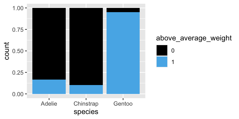


# Numerical breakdown of weight within species
penguins %>%
  drop_na(above_average_weight) %>%
  tabyl(species, above_average_weight) %>%
  adorn_percentages("row") %>%
  adorn_ns()
##    species                0               1
##     Adelie 0.83443709 (126) 0.1655629  (25)
##  Chinstrap 0.89705882  (61) 0.1029412   (7)
##     Gentoo 0.04878049   (6) 0.9512195 (117)

Suppose we come across a penguin that’s below average weight ($X_1 = 0$). For what species is this most likely? RECALL: $L(Y | X_1 = 0) = P(X_1 = 0 | Y)$.

$Y$	$A$	$C$	$G$	Total
$L(Y \| X_1 = 0)$	0.8344	0.8971	0.0488	1.7803

WARM-UP 2

Verify the following posterior model for the penguin’s species ($Y$) given that they’re below average weight, $X_1 = 0$.

$Y$	$A$	$C$	$G$	Total
$P(Y \| X_1 = 0)$	0.654	0.315	0.031	1

WARM-UP 3

What if, instead, we classified a penguin’s species ($Y$) based on its bill length ($X_2$) alone? For example, suppose we come across a penguin with a 50mm long bill.

For what species are we most likely to observe this bill length?
How might we calculate $L(Y | X_2 = 50)$? NOTE: Since $X_2$ is quantitative and continuous, this is different than our approach to calculating the likelihood when $X_1$ was a discrete categorical variable.

# Graphical breakdown of bill length within species
ggplot(penguins, aes(x = bill_length_mm, fill = species)) +
  geom_density(alpha = 0.7) +
  geom_vline(xintercept = 50, linetype = "dashed")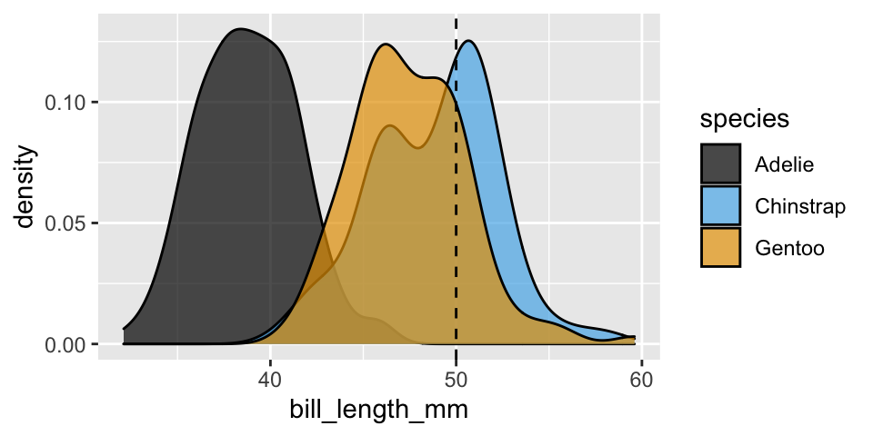

15.2 Exercises

GOAL

Use naive Bayes classification to classify a categorical response variable $Y$ (with 2+ categories) using any combination of categorical or quantitative predictors $X$. NOTE: You will first do this from scratch, and then use a shortcut function. Taking the time to do this isn’t some random tedious exercise. It makes the difference between kind of understanding how the algorithm works and really understanding how it works.
Explore the pros and cons of naive Bayes classification.
Compare the classification performance of naive Bayes vs logistic regression.

Calculating the likelihood
Again, suppose we come across a penguin with a 50mm long bill, $X_2 = 50$. To update our posterior understanding of the penguin’s species $Y$, we have to calculate the likelihood of observing a 50mm long bill for each species: $L(Y | X_2 = 50)$. Since $X_2$ is quantitative, the typical assumption in naive Bayesian classification is that $X_2$ is Normally distributed within each $Y$ category, i.e. species, but with possibly different means and standard deviations:

\[\begin{split} X_2 | (Y = \text{Adelie}) & \sim N(\mu_A, \sigma_A^2) \\ X_2 | (Y = \text{Chinstrap}) & \sim N(\mu_C, \sigma_C^2) \\ X_2 | (Y = \text{Gentoo}) & \sim N(\mu_G, \sigma_G^2) \\ \end{split}\]
1. Calculate the mean and standard deviation of bill_length_mm within each of the 3 species. These are our simple estimates of the means ($\mu_A, \mu_C, \mu_G$) and standard deviations ($\sigma_A, \sigma_C, \sigma_G$). NOTE: You’ll need to use drop_na(bill_length_mm).
2. Plot the tuned Normal models for each species. Is the Normal assumption reasonable in our example, or is it too naive?
```
ggplot(penguins, aes(x = bill_length_mm, color = species)) +
  geom_density(aes(fill = species), alpha = 0.25) +
  stat_function(fun = dnorm, args = list(mean = 38.8, sd = 2.66),
                aes(color = "Adelie")) +
  stat_function(fun = dnorm, args = list(mean = 48.8, sd = 3.34),
                aes(color = "Chinstrap")) +
  stat_function(fun = dnorm, args = list(mean = 47.5, sd = 3.08),
                aes(color = "Gentoo")) +
  geom_vline(xintercept = 50, linetype = "dashed")
```
3. The likelihoods $L(Y | X_2 = 50)$ are defined by the values of the Normal density curve when $X_2 = 50$. Calculate these likelihoods. The one for Adelie is provided as an example.
```
# L(Y = A | X_2 = 50)
dnorm(50, mean = 38.8, sd = 2.66)

# L(Y = C | X_2 = 50)

# L(Y = G | X_2 = 50)
```
4. Based on the likelihood values, for which species is a 50mm bill length most likely?

Posterior model
Our prior understanding was that the penguin was most likely an Adelie. But the data (a 50mm bill length) is most consistent with Chinstraps. The posterior model balances these 2 conflicting pieces of evidence:

$Y$ $A$ $C$ $G$

$P(Y | X_2 = 50)$ 0.0002 0.3972 0.6026
1. Confirm the posterior calculation for the Chinstrap species. Your answer may be a bit off due to rounding.
2. How would you classify this penguin based on its bill length alone?

\(Y\)	\(A\)	\(C\)	\(G\)
\(P(Y \| X_2 = 50)\)	0.0002	0.3972	0.6026

Two predictors
1. Construct a visualization of the relationship between species ($Y$) and bill_length_mm ($X_2$) alone. (Hint: We did this above.) If we only have information about bill length, is it easy to distinguish between species? If not, which species might we have a tough time distinguishing between?
2. Construct a visualization of the relationship between species ($Y$) and flipper_length_mm ($X_3$) alone. If we only have information about flipper length, is it easy to distinguish between species? If not, which species might we have a tough time distinguishing between?
3. Suppose we’re able to take 2 penguin measurements, both bill_length_mm ($X_2$) and flipper_length_mm ($X_3$). Construct a visualization of the relationship of species ($Y$) with bill length ($X_2$) and flipper length ($X_3$). If we only have information about flipper length, is it easy to distinguish between species? If not, which species might we have a tough time distinguishing between?

Likelihoods with 2 predictors
Suppose we come across a penguin with a 50mm long bill and a 195mm long flipper.
1. Based on your plot in part c above, with what species are these features most consistent?
2. To formalize this observation, we can calculate the likelihood of observing this combination of features. To this end, naive Bayes classification assumes that predictors are conditionally independent, thus
  
  \[L(Y | X_2 = 50, X_3 = 195) = L(Y | X_2 = 50)L(Y | X_3 = 195)\]
  
  That is, within each species, we assume that a penguin’s bill length is unrelated to its flipper length. Based on your plot in part c above, is this a reasonable assumption or is it naive?

Calculate the likelihood
Calculate the likelihood for each species $L(Y | X_2 = 50, X_3 = 195) = L(Y | X_2 = 50)L(Y | X_3 = 195)$. HINT: Before filling in the blanks, you’ll need to determine the assumed Normal models of flipper length within each species.

# # L(Y = A | X_2 = 50)L(Y = A | X_3 = 195)
# dnorm(50, mean = 38.8, sd = 2.66) * ___
# 
# # L(Y = C | X_2 = 50)L(Y = C | X_3 = 195)
# dnorm(50, mean = 48.8, sd = 3.34) * ___
# 
# # L(Y = G | X_2 = 50)L(Y = G | X_3 = 195)
# dnorm(50, mean = 47.5, sd = 3.08) * ___

Posterior model
Our prior understanding was that the penguin was most likely an Adelie. But the data (a 50mm long bill and 195mm long flipper) is most consistent with Chinstraps. The posterior model balances these 2 conflicting pieces of evidence:

$Y$ $A$ $C$ $G$

$P(Y | X_2 = 50, X_3 = 195)$ 0.0003 0.9944 0.0052
1. Confirm the posterior calculation for the Chinstrap species. Your answer may be a bit off due to rounding.
2. How would you classify this penguin based on its bill length and flipper length? How does this compare to your classification based on bill length alone (that the penguin was Gentoo)?

\(Y\)	\(A\)	\(C\)	\(G\)
\(P(Y \| X_2 = 50, X_3 = 195)\)	0.0003	0.9944	0.0052

Naive Bayes classification in R
It was an important exercise to implement the naive Bayes algorithm from scratch. But now that we know how it works, let’s use the shortcut naiveBayes() function in the e1071 package.
1. First, run the naive Bayes algorithm using data on bill length alone:
```
# Load the package
library(e1071)

# Run the algorithm using only data on bill length
naive_model_1 <- naiveBayes(species ~ bill_length_mm, data = penguins)
```
  Then use this to classify our penguin with a 50mm long bill and 195mm long flipper (where the latter piece of info is ignored by this algorithm). How does this result compare to the one you made from scratch in exercise 2?
```
# Define our penguin
our_penguin <- data.frame(bill_length_mm = 50, flipper_length_mm = 195)

# Predict the species using bill length alone
predict(naive_model_1, newdata = our_penguin, type = "raw")
```
2. Next, run the naive Bayes classification algorithm using information about both bill length and flipper length. Call this naive_model_2. Then use this to classify our penguin with a 50mm long bill and 195mm long flipper. How does this result compare to the one you made from scratch in exercise 6?

Classification regions
Essentially, naive Bayes classification (as well as logistic regression and other classification methods) produces classification regions – classifications of $Y$ are based on the region that the observed predictor values fall into. For example, plot and discuss the classification regions defined by naive_model_2. How well do these reflect the true penguin species?

# Define a grid of data points with different bill and flipper lengths
# Classify / predict the species for each data point
grid_data <- expand_grid(
    bill_length_mm = seq(30, 60, length = 100),
    flipper_length_mm = seq(170, 240, length = 100)) %>%
  mutate(classification = predict(naive_model_2, newdata = .))

# Plot the classification regions
ggplot(grid_data, aes(x = flipper_length_mm, y = bill_length_mm, color = classification)) +
  geom_point(alpha = 0.2)

# Plot where the observed data falls among the classification regions
ggplot(grid_data, aes(x = flipper_length_mm, y = bill_length_mm, color = classification)) +
  geom_point(alpha = 0.2) + 
  geom_point(data = penguins, aes(x = flipper_length_mm, y = bill_length_mm, color = species))

Evaluating the naive Bayes classifications: part 1
As with any model, we need to consider the fairness, wrongness, and classification accuracy of our naive Bayes algorithms. Let’s focus on classification accuracy.
1. Use the naive_classification_summary_cv() function in the bayesrules package to evaluate the (cross-validated) classification accuracy of our algorithm which used data on bill length alone:
```
set.seed(84735)
naive_classification_summary_cv(
  model = naive_model_1, data = penguins, y = "species", k = 10)$cv
```
2. What’s the cross-validated overall accuracy rate? NOTE: You’ll need to do some arithmetic.
3. For which species are this algorithm’s the most accurate? The least accurate?

Evaluating the naive Bayes classifications: part 2
1. Obtain the (cross-validated) classification accuracy of our algorithm which used data on both bill length and flipper length.
2. What’s the cross-validated overall accuracy rate of this algorithm?
3. For which species are this algorithm’s the most accurate? The least accurate?
4. If you could only pick 1 algorithm for classifying penguin species, which would you pick, that which used only bill length or that which used both bill length and flipper length?

Pros and cons
1. Name two pros of the naive Bayes classification algorithm. For example: What can it do that logistic regression can’t? What was your experience when implementing the naiveBayes() function vs the stan_glm() function?
2. In terms of cons, identify two things that are “naive” about the naive Bayes classification algorithm.
3. As another point, notice that the naive Bayes classification algorithm gave you some final classifications, but it didn’t have any coefficients (eg: $\beta$). Why is this a “con?”

naive Bayes vs logistic regression
When $Y$ is a binary categorical response variable, we can use both logistic regression or naive Bayes classification to classify $Y$. For example, suppose we wish to classify whether a news article is_fake $Y$ based on its number of title_words $X_1$ and title_has_excl $X_2$ (whether the title includes an exclamation point).
1. Use both Bayesian logistic regression (with weakly informative priors) and naive Bayes classification to classify whether an article is_fake. Obtain cross-validated summaries of the posterior classification accuracy for these 2 algorithms.
2. In terms of posterior classification, which method was more accurate?
3. Can you think of a situation where you’d want to use logistic regression in this example, even if the naive Bayes classifications were more accurate?

15.3 Totally optional

In some settings, we have a categorical response variable $Y$ with more than 2 categories! Though we can apply the naive Bayes algorithm in these settings, we can’t apply Bayesian logistic regression or even a Beta-Binomial model (both of which assume $Y$ is binary). For fun, consider the multinomial extension of the Beta-Binomial:

\[\begin{split} (Y_1,Y_2,...,Y_k) & \sim \text{Multinomial}(n,\pi_1,\pi_2,...,\pi_k) \\ (\pi_1,\pi_2,...,\pi_k) & \sim \text{Dirichlet}(\alpha_1,\alpha_2,...,\alpha_k) \\ \end{split}\]

For a little example, suppose 3 candidates were running for president. Let $\pi_1,\pi_2,\pi_3$ be the proportion of people that plan to vote for each candidate ($\pi_1+\pi_2+\pi_3 = 1$).

Suppose you have the following prior model for the candidates’ support: \[(\pi_1,\pi_2,\pi_3) \sim \text{Dirichlet}(1,2,3)\] Explain in words what this model indicates about your prior understanding. Include measurements of the prior means $E(\pi_i)$. NOTE: You’ll have to do some research on the Dirichlet model!

In a poll of 1000 people, suppose $Y_1 = 600$ support candidate 1, $Y_2 = 300$ support candidate 2, and $Y_3 = 100$ support candidate 3. In light of this data, build your posterior model of $(\pi_1,\pi_2,\pi_3)$. Be sure to specify its name and any parameters upon which it depends. NOTE: You’ll have to do some research on the Multinomial model!
\[\begin{split} (Y_1,Y_2,Y_3) & \sim \text{Multinomial}(1000,\pi_1,\pi_2,\pi_3) \\ (\pi_1,\pi_2,\pi_3) & \sim \text{Dirichlet}(1,2,3) \\ \end{split} \;\; \Rightarrow \;\; (\pi_1,\pi_2,\pi_3) | (Y_1=600,Y_2=300,Y_3=100) \sim ???\]

Interpret what your posterior model indicates about your updated understanding of the candidates’ support. Include measurements of the posterior means $E(\pi_i|Y)$.

In general:
1. Build the posterior model of $(\pi_1,\pi_2,...,\pi_k)$ for the Multinomial-Dirichlet model: \[\begin{split} (Y_1,Y_2,...,Y_k) & \sim \text{Multinomial}(n,\pi_1,\pi_2,...,\pi_k) \\ (\pi_1,\pi_2,...,\pi_k) & \sim \text{Dirichlet}(\alpha_1,\alpha_2,...,\alpha_k) \\ \end{split}\]
2. How can we tune the Dirichlet prior to be vague?

15.4 Solutions

Calculating the likelihood

penguins %>%
  drop_na(bill_length_mm) %>%
  group_by(species) %>%
  summarize(mean(bill_length_mm), sd(bill_length_mm))
## # A tibble: 3 x 3
##   species   `mean(bill_length_mm)` `sd(bill_length_mm)`
##   <fct>                      <dbl>                <dbl>
## 1 Adelie                      38.8                 2.66
## 2 Chinstrap                   48.8                 3.34
## 3 Gentoo                      47.5                 3.08

Seems reasonable.

ggplot(penguins, aes(x = bill_length_mm, color = species)) +
  geom_density(aes(fill = species), alpha = 0.25) +
  stat_function(fun = dnorm, args = list(mean = 38.8, sd = 2.66),
                aes(color = "Adelie")) +
  stat_function(fun = dnorm, args = list(mean = 48.8, sd = 3.34),
                aes(color = "Chinstrap")) +
  stat_function(fun = dnorm, args = list(mean = 47.5, sd = 3.08),
                aes(color = "Gentoo")) +
  geom_vline(xintercept = 50, linetype = "dashed")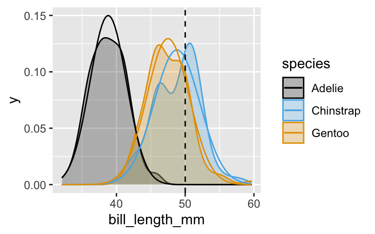

# L(Y = A | X_2 = 50)
dnorm(50, mean = 38.8, sd = 2.66)
## [1] 2.119955e-05

# L(Y = C | X_2 = 50)
dnorm(50, mean = 48.8, sd = 3.34)
## [1] 0.1119782

# L(Y = G | X_2 = 50)
dnorm(50, mean = 47.5, sd = 3.08)
## [1] 0.09317395

Chinstrap. $L(Y = C | X_2 = 50) > L(Y = G | X_2 = 50) > L(Y = A | X_2 = 50)$.

Posterior model

0.19767*0.112 / (0.44186*0.00002 + 0.19767*0.112 + 0.36047*0.0932)
## [1] 0.3971578

Gentoo.

Two predictors

It’s tough to distinguish between Gentoo and Chinstrap based on bill length alone.

ggplot(penguins, aes(x = bill_length_mm, fill = species)) + 
  geom_density(alpha = 0.5)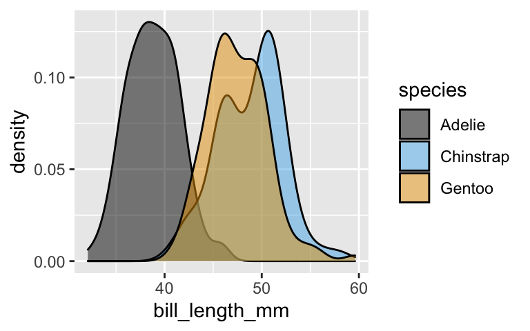

It’s tough to distinguish between Adelie and Chinstrap based on flipper length alone.

ggplot(penguins, aes(x = flipper_length_mm, fill = species)) + 
  geom_density(alpha = 0.5)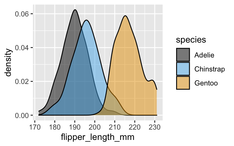

The species are fairly distinct when considering both bill length and flipper length.

ggplot(penguins, aes(x = flipper_length_mm, y = bill_length_mm, color = species)) + 
  geom_point()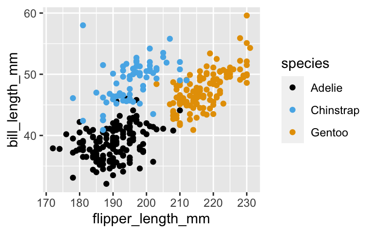

Likelihoods with 2 predictors
1. Chinstrap
2. Not really. Within each species, there’s a positive association between bill and flipper length.

Calculate the likelihood

# Calculate the mean and sd of flipper length within each species
penguins %>%
  drop_na(flipper_length_mm) %>%
  group_by(species) %>%
  summarize(mean(flipper_length_mm), sd(flipper_length_mm))
## # A tibble: 3 x 3
##   species   `mean(flipper_length_mm)` `sd(flipper_length_mm)`
##   <fct>                         <dbl>                   <dbl>
## 1 Adelie                         190.                    6.54
## 2 Chinstrap                      196.                    7.13
## 3 Gentoo                         217.                    6.48

# L(Y = A | X_2 = 50)L(Y = A | X_3 = 195)
dnorm(50, mean = 38.8, sd = 2.66) * dnorm(195, mean = 190, sd = 6.54)
## [1] 9.654647e-07

# L(Y = C | X_2 = 50)L(Y = C | X_3 = 195)
dnorm(50, mean = 48.8, sd = 3.34) * dnorm(195, mean = 196, sd = 7.13)
## [1] 0.006204155

# L(Y = G | X_2 = 50)L(Y = G | X_3 = 195)
dnorm(50, mean = 47.5, sd = 3.08) * dnorm(195, mean = 217, sd = 6.48)
## [1] 1.801748e-05

Posterior model

0.19767*0.006204155 / (0.44186*0.000000965 + 0.19767*0.006204155 + 0.36047*0.000018)
## [1] 0.9943932

Chinstrap. Based on bill length alone, we classified it as Gentoo.

Naive Bayes classification in R

This matches our work from scratch.

# Load the package
library(e1071)

# Run the algorithm using only data on bill length
naive_model_1 <- naiveBayes(species ~ bill_length_mm, data = penguins)

# Define our penguin
our_penguin <- data.frame(bill_length_mm = 50, flipper_length_mm = 195)

# Predict the species using bill length alone
predict(naive_model_1, newdata = our_penguin, type = "raw")
##            Adelie Chinstrap    Gentoo
## [1,] 0.0001690279 0.3978306 0.6020004

# Run the algorithm using only data on bill length & flipper length
naive_model_2 <- naiveBayes(species ~ bill_length_mm + flipper_length_mm, data = penguins)

# Predict the species
predict(naive_model_2, newdata = our_penguin, type = "raw")
##            Adelie Chinstrap      Gentoo
## [1,] 0.0003445688 0.9948681 0.004787365

Classification regions

# Define a grid of data points with different bill and flipper lengths
# Classify / predict the species for each data point
grid_data <- expand_grid(
    bill_length_mm = seq(30, 60, length = 100),
    flipper_length_mm = seq(170, 240, length = 100)) %>%
  mutate(classification = predict(naive_model_2, newdata = .))

# Plot the classification regions
ggplot(grid_data, aes(x = flipper_length_mm, y = bill_length_mm, color = classification)) +
  geom_point(alpha = 0.2)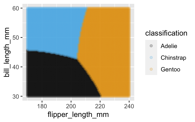


# Plot where the observed data falls among the classification regions
ggplot(grid_data, aes(x = flipper_length_mm, y = bill_length_mm, color = classification)) +
  geom_point(alpha = 0.2) + 
  geom_point(data = penguins, aes(x = flipper_length_mm, y = bill_length_mm, color = species))

Evaluating the naive Bayes classifications: part 1

set.seed(84735)
naive_classification_summary_cv(
  model = naive_model_1, data = penguins, y = "species", k = 10)$cv
##    species       Adelie Chinstrap       Gentoo
##     Adelie 95.39% (145) 0.00% (0)  4.61%   (7)
##  Chinstrap  5.88%   (4) 7.35% (5) 86.76%  (59)
##     Gentoo  7.26%   (9) 4.84% (6) 87.90% (109)

75.3%

(145 + 5 + 109) / (145 + 0 + 7 + 4 + 5 + 59 + 9 + 6 + 109)
## [1] 0.752907

most accurate: Adelie. least accurate: Chinstrap (which is commonly misclassified as Gentoo)

Evaluating the naive Bayes classifications: part 2

set.seed(84735)
naive_classification_summary_cv(
  model = naive_model_2, data = penguins, y = "species", k = 10)$cv
##    species       Adelie   Chinstrap       Gentoo
##     Adelie 96.05% (146)  2.63%  (4)  1.32%   (2)
##  Chinstrap  7.35%   (5) 86.76% (59)  5.88%   (4)
##     Gentoo  0.81%   (1)  0.81%  (1) 98.39% (122)

76%

(145 + 7 + 108) / (145 + 4 + 2 + 5 + 59 + 4 + 0 + 1 + 122)
## [1] 0.7602339

most accurate: Gentoo. least accurate: Chinstrap.
I’d pick the 2nd one. It maintains high overall accuracy and is much better at detecting Chinstrap, without drastic consequence to classifying the other 2 species.

Pros and cons
1. - naive Bayes works for categorical $Y$ variables with 2+ categories
  - naive Bayes is computationally efficient (doesn’t require MCMC)
2. - it assumes that all quantitative predictors are normally distributed within each $Y$ category
  - it assumes conditional independence, i.e. that predictors are independent within each $Y$ category
3. naive Bayes classification might give us accurate predictions, but it doesn’t give us a sense of where they come from (no regression formula) or of how $Y$ is related to the predictors.

naive Bayes vs logistic regression
Try this on your own!