10 Bayesian regression

GOALS

Build a Bayesian regression model of response variable \(Y\) by predictor variable \(X\), one step at a time.
Interpret and simulate Bayesian regression priors.
Conduct a posterior regression analysis.
Start thinking about how to evaluate a Bayesian regression model.

RECOMMENDED READING

Bayes Rules! Chapter 9.

Why Bayesian regression?

Compared to frequentist regression…

we can formally incorporate prior expertise (which is especially important when we don’t have much data);
we can naturally and sequentially update our model as more data come in; and
the analysis answers more natural questions.

Close-to-home examples of Bayesian modeling

Raven McKnight (’20) used Bayesian spatial transit models at Metro Transit.
Sofia Pozsonyiova (’20) is starting her research in Bayesian biomedical statistics at Duke University (a largely Bayesian institution).
Johnny Paige (’14), whose work spans Bayesian spatial statistics and MCMC methodology, is starting a postdoc at the Norwegian Institute of Science and Technology.
Susan Fox uses AI tools powered by Bayesian statistics

10.1 Warm-up

WARM-UP 1: Just \(Y\)

Suppose we’re interested in the afternoon temperature in Perth, Australia. What’s an appropriate model for the variability in 3pm temperature, \(Y\), from day to day?

\(Y | \pi \sim \text{Bin}(1000, \pi)\)
\(Y | \lambda \sim \text{Pois}(\lambda)\)
\(Y | \mu, \sigma \sim N(\mu, \sigma^2)\)

WARM-UP 2: Adding a predictor

Suppose we wished to predict a day’s 3pm temperature from its 9am temperature, \(X\). To this end, assume that 3pm temperature is linearly dependent on 9am temperature:

\[Y = E(Y|X) + \varepsilon = \beta_0 + \beta_1 X + \varepsilon\]

Modify your model from the first warm-up example to incorporate the 9am temperature predictor \(X\).

WARM-UP 3: Finalizing the Bayesian model

Upon what parameters does your model depend? NOTE: \(Y\) and \(X\) are “data variables,” not parameters.
What are appropriate prior models for these parameters (e.g. Beta, Gamma, Normal)?

The Bayesian Normal regression model

To model response variable \(Y\) by predictor \(X\), suppose we collect \(n\) data points. Let \((Y_i, X_i)\) denote the observed data on each case \(i \in \{1, 2, \ldots, n\}\). Then the Bayesian Normal regression model is as follows:

\[\begin{split} Y_i | \beta_0, \beta_1, \sigma & \stackrel{ind}{\sim} N(\mu_i, \sigma^2) \;\; \text{ where } \mu_i = \beta_0 + \beta_1 X_i\\ \beta_{0c} & \sim N(m_0, s_0^2) \\ \beta_1 & \sim N(m_1, s_1^2) \\ \sigma & \sim \text{Exp}(l) \\ \end{split}\]

NOTES:

Equivalently, we can write the data model as
\[Y_i = \beta_0 + \beta_1 X_i + \varepsilon_i \;\; \text{ where } \;\; \varepsilon_i \stackrel{ind}{\sim} N(0, \sigma^2)\] Without the priors, this is what you studied in STAT 155!
\(\sigma\) measures the typical deviation of an observed \(Y\) from the regression line \(\beta_0 + \beta_1 X\).
The priors on \((\beta_0, \beta_1, \sigma)\) are independent of one another.
For interpretability, we state our prior understanding of the model intercept \(\beta_0\) through the centered intercept \(\beta_{0c}\). Whereas \(\beta_0\) measures the typical \(Y\) value when \(X = 0\) (which is often contextually infeasible), \(\beta_{0c}\) measures the typical \(Y\) value at the typical \(X\) value.
There are other prior models we might use, but those here are the default in rstanarm.

Studying the regression posterior

For observed data \(\vec{y}\) and \(\vec{x}\), our goal is to examine the posterior model of the regression parameters:

\[(\beta_0,\beta_1,\sigma) | (\vec{y}, \vec{x}) \; \sim \; ???\] This requires simulation! Why? The posterior pdf is

\[\begin{split} f(\beta_0,\beta_1,\sigma \; | \; \vec{y}) & \propto f(\vec{y} | \beta_0, \beta_1, \sigma) f(\beta_0, \beta_1,\sigma) \\ & = \left[\prod_{i=1}^{n}f(y_i|\beta_0, \beta_1, \sigma) \right] \cdot f(\beta_0) f(\beta_1) f(\sigma) \\ \end{split}\]

where for \(y_i \in (-\infty,\infty)\), \(\beta_j \in (-\infty,\infty)\), and \(\sigma \in (0,\infty)\):

\[\begin{split} f(y_i|\beta_0,\beta_1,\sigma) & = \sqrt{\frac{1}{2\pi\sigma^2}} \exp\left\lbrace-\frac{1}{2\sigma^2} (y_i - (\beta_0+\beta_1x_{i1}))^2 \right\rbrace \\ f(\beta_j) & = \sqrt{\frac{1}{2\pi s_j^2}} \exp\left\lbrace-\frac{1}{2 s_j^2} (\beta_j - m_j)^2 \right\rbrace \\ f(\sigma) & = l e^{-l\sigma} \\ \end{split}\]

10.2 Exercises

NOTE

Since much of the syntax is new and so that you can focus on the concepts, most R code has been given to you. Be sure to still pause and check it out so that you can call upon it when needed in the future.

The story

Consider the following Bayesian regression model of 3pm temperature \(Y\) vs 9am temperature \(X\):

\[\begin{split} Y_i | \beta_0, \beta_1, \sigma & \stackrel{ind}{\sim} N(\mu_i, \sigma^2) \;\; \text{ where } \mu_i = \beta_0 + \beta_1 X_i\\ \beta_{0c} & \sim N(30, 7^2) \\ \beta_1 & \sim N(2, 1^2) \\ \sigma & \sim \text{Exp}(0.1) \\ \end{split}\]

To learn about this relationship, we’ll use data on Perth, Australia from the bayesrules package. Load this data along with some handy packages:

# Load packages
library(tidyverse)
library(tidybayes)
library(rstan)
library(rstanarm)
library(bayesplot)
library(bayesrules)
library(broom.mixed)

# Load data
data("weather_perth")

Interpreting the prior models
Let’s start by interpreting the prior models of \(\beta_{0c}\), \(\beta_1\), and \(\sigma\). In doing so, it’s important to also keep track of what these parameters mean in the context of our analysis.
1. What’s our prior understanding of \(\beta_{0c}\), the typical 3pm temperature on a day with a typical morning temperature?
```
plot_normal(30, 7) +
          labs(x = expression(beta[0]), y = "density")
```
2. What does the \(\beta_1\) prior indicate about our understanding of how 3pm temperature changes with 9am temperature?
```
plot_normal(2, 1) +
          labs(x = expression(beta[1]), y = "density")
```
3. What does the \(\sigma\) prior indicate about our understanding of how much the observed 3pm temperatures might vary on days with the same 9am temperatures?
```
plot_gamma(1, 0.1) +
          labs(x = expression(sigma), y = "density")
```

Prior simulation
The prior models help us understand each individual parameter \(\beta_{0c}\), \(\beta_1\), and \(\sigma\). To better understand how these work together in the model of 3pm temperatures, we can simulate a sample of prior plausible parameter sets using the stan_glm() function in the rstanarm package:
```
# Simulate the prior model
temp_prior <- stan_glm(
  temp3pm ~ temp9am, data = weather_perth,
  family = gaussian,
  prior_intercept = normal(30, 7),
  prior = normal(2, 1),
  prior_aux = exponential(0.1),
  prior_PD = TRUE,
  chains = 4, iter = 5000*2, seed = 84735)
```
Only if your code broke in the previous chunk, import the prior simulation results:
```
temp_prior <- readRDS(url("https://www.macalester.edu/~ajohns24/data/stat454/weather_prior_1.rds"))
```
Check out the stan_glm() syntax. Summarize the purpose of each set of lines:
- temp3pm ~ temp9am, data = weather_perth and family = gaussian
- prior_intercept = normal(30, 7) and prior = normal(2, 1) and prior_aux = exponential(0.1)
  - prior_PD = TRUE
  - chains = 4, iter = 5000*2, seed = 84735

Prior check
temp_prior contains 20,000 prior plausible parameter sets \((\beta_{0c}, \beta_1, \sigma)\):
```
# Check out the first 6 parameter sets
as.data.frame(temp_prior) %>%
  head()
```
It’s important to check our priors to make sure they’re tuned appropriately (and that we understand them!).
1. First, consider what type of 3pm temperatures our prior models would expect. Simulate and plot 50 separate samples of 3pm temperatures, 1 from each of 50 separate prior plausible parameter sets in temp_prior. Note the range, distributions, and differences among the 50 samples. Do these indicate that the priors are informative, vague, or somewhere in between? Why?
```
# Plot a prior predictive check
pp_check(temp_prior) +
  xlab("3pm temperature")
```
2. Let’s also consider our prior understanding of the linear relationships between 3pm and 9am temperatures. The following chunk simulates 200 prior plausible regression lines \(\beta_0 + \beta_1 X\), 1 from each of 200 prior plausible parameter sets in temp_prior. Run it a few times and summarize your observations.
```
# 200 prior model lines
weather_perth %>%
  add_fitted_draws(temp_prior, n = 200) %>%
  ggplot(aes(x = temp9am, y = temp3pm)) +
    geom_line(aes(y = .value, group = .draw), alpha = 0.15)
```
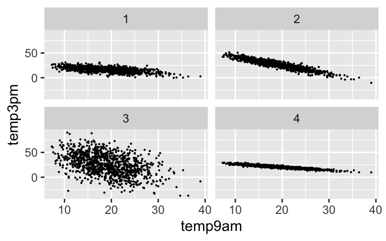
  1. The plot in part b illuminates prior plausible regression lines \(\beta_0 + \beta_1 X\). To explore our prior understanding of potential variability from this line, \(\sigma\), the following chunk simulates 4 prior plausible sets of temperature data, 1 from each of 4 prior plausible parameter sets in temp_prior. Run it a few times and summarize your observations.
```
# Plot 4 prior simulated datasets
weather_perth %>%
  add_predicted_draws(temp_prior, n = 4) %>%
  ggplot(aes(x = temp9am, y = temp3pm)) +
    geom_point(aes(y = .prediction, group = .draw), size = 0.1) +
    facet_wrap(~ .draw)
```

Simulate the posterior & perform simulation diagnostics
Next, let’s simulate the posterior. We don’t have to start from scratch. Rather, we can update() our prior simulation using prior_PD = FALSE. Further, to ensure that we can “trust” the MCMC posterior simulation results, check out trace plots and density plots of the multiple chains.
```
# Simulate the posterior
temp_posterior <- update(temp_prior, prior_PD = FALSE)

# Perform MCMC diagnostics
```
Only if you get errors in the above code, import the posterior simulation results:
```
temp_posterior <- readRDS(url("https://www.macalester.edu/~ajohns24/data/stat454/weather_posterior_1.rds"))
```

Posterior analysis
1. Just as we did for the prior, we can better understand our posterior model by simulating 50 posterior plausible regression lines \(\beta_0 + \beta_1 X\). Run this chunk a few times. Summarize your observations as well as how our understanding evolved from the prior to the posterior.
```
## 50 simulated posterior model lines
#___ %>%
#  ___(___, n = 50) %>%
#  ggplot(aes(x = ___, y = ___)) +
#    geom_line(aes(y = ___, group = ___), alpha = 0.15) +
#    geom_point(data = weather_perth, size = 0.05)
```
2. Check out a posterior summary table. Do we have ample evidence of a positive association between 3pm and 9am temperatures, i.e. that the warmer it is in the morning, the warmer it tends to be in the afternoon? Explain.
```
# Get posterior summaries of the "fixed" parameters (betas)
# and "auxiliary" parameter (sigma)
tidy(temp_posterior, effects = c("fixed", "aux"),
     conf.int = TRUE, conf.level = 0.80)
```

Posterior prediction: from scratch
Suppose it’s 20 degrees at 9am. Simulate, plot, and describe a posterior predictive model for the 3pm temperature. HINTS:

Predict a 3pm temperature from each of the 20,000 parameter sets \((\beta_0, \beta_1, \sigma)\).
To work with (Intercept), put a backtick at the start and end.

## Store the MCMC chains as a data frame
# temp_chains <- as.data.frame(temp_posterior)
#
## Simulate the posterior predictive model
# set.seed(84735)
# predict_20 <- ___ %>% 
#   ___(y_prediction = ___)
# 
## Plot the posterior predictive model
# ggplot(predict_20, aes(x = ___)) + 
#   geom_density()

Posterior prediction: shortcut
It’s important to understand where the predictions come from. BUT there’s also a shortcut. Use the posterior_predict() function to simulate the posterior predictive model of 3pm temperature when it’s 20 degrees at 9am. Further, use posterior_interval() and mcmc_dens() to summarize the posterior. Examine the results and confirm that they’re similar to your “from scratch” simulation.

# Simulate a set of predictions
set.seed(84735)
shortcut_prediction <- posterior_predict(
    temp_posterior, newdata = data.frame(temp9am = 20))

# Construct a 90% posterior credible interval
posterior_interval(shortcut_prediction, prob = 0.9)

# Plot the approximate predictive model
mcmc_areas(shortcut_prediction, prob = 0.9) + 
  scale_x_continuous(breaks = seq(15, 35, by = 5)) + 
  xlab("3pm temperature")

Posterior prediction follow-up
Evaluating Bayesian predictions is a bit different than evaluating frequentist predictions. For example, suppose today’s temperature in Perth was 20 degrees at 9am and 16 degrees at 3pm. Come up with 2 approaches to measuring / indicating the quality of our prediction for this particular day. HINT: For context, reexamine the mcmc_areas() plot.

Using weakly informative priors
Unless we have specific prior information or expertise, we can use weakly informative default priors in stan_glm(). Unlike flat or vague priors which would give prior weight to non-sensible parameter values, weakly informative priors reflect general prior uncertainty about sensible model parameters. For example, a flat prior assumes that a typical 3pm temperature of -1000 degrees on days with the typical temperature (\(\beta_{0c}\)) is just as plausible as a 40 degree temperature. Weakly informative priors do not. These are tuned by stan_glm() using basic information about the scales of our data variables, but no information about the relationship among these variables.
1. Simulate the default prior models using stan_glm(). NOTE: You’ll need to eliminate 3 lines from the original stan_glm() code in exercise 2.
2. To learn how the prior models were tuned, check out prior_summary(YOUR_MODEL_FROM_PART_a). Summarize the tunings reported by the Adjusted prior terms.
3. Examine the prior for the temp9am coefficient. Where is this centered and, in the context of a regression analysis, why is this a “vague” or “weakly informative” choice?
4. Perform a complete prior check (see exercise 3). Summarize how the weakly informative priors compare to our original priors.

Model evaluation
Of course, before applying or reporting any model, we must evaluate its quality. Name 2 or 3 questions that are important to ask about our model. If relevant, try to answer these questions using your original posterior simulation results.

Your turn
There was a lot of new syntax. To practice, perform a Bayesian analysis of the relationship between temp3pm and humidity9am.

10.3 Solutions

Interpreting the prior models
1. The typical 3pm temperature on a day with a typical morning temperature is likely around 30 degrees, but could be anywhere between 10 and 50 degrees.
```
plot_normal(30, 7) +
          labs(x = expression(beta[0]), y = "density")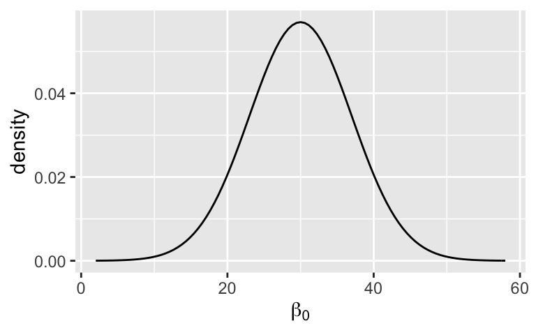
```
2. We expect that 3pm temperature most likely increases with 9am temperature, somewhere between 0 and 4 additional degrees per 1 degree increase in 9am temperature. But we’re not sure – there could also be no relationship (\(\beta_1 = 0\) is within the realm of prior possibilities).
```
plot_normal(2, 1) +
          labs(x = expression(beta[1]), y = "density")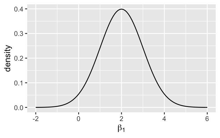
```
3. We think that, on days with the same 9am temperature, the standard deviation in 3pm temperatures is somewhere below 30 rides.
```
plot_gamma(1, 0.1) +
          labs(x = expression(sigma), y = "density")
```

Prior simulation
Code provided.

Prior check

# Check out the first 6 parameter sets
as.data.frame(temp_prior) %>%
  head()
##   (Intercept)  temp9am     sigma
## 1  -29.281855 2.819044  6.488199
## 2   -6.621373 1.766838  3.502557
## 3    3.415011 1.383317  4.625897
## 4    5.619093 1.305730  4.183584
## 5   -5.056828 1.841504  2.756084
## 6    7.568718 1.501633 12.389273

The prior simulations of 3pm temperature range from -25 to 100. This is very wide on the Celsius scale, however elimates unrealistic temperatures (eg: 1000 degrees). Thus the priors seem somewhere between vague and informative.
```
# Plot a prior predictive check
pp_check(temp_prior) +
  xlab("3pm temperature")
```

Most of the model lines are positive, reflecting a prior assumption of a positive association between afternoon and morning temperatures. However, the slopes and intercepts are quite varied.

# 200 prior model lines
weather_perth %>%
  add_fitted_draws(temp_prior, n = 200) %>%
  ggplot(aes(x = temp9am, y = temp3pm)) +
    geom_line(aes(y = .value, group = .draw), alpha = 0.15)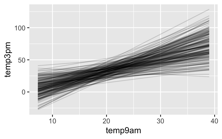

Notice the variety in slopes, intercepts, and strengths of the relationship (the last of these reflecting \(\sigma\)).

# Plot 4 prior simulated datasets
weather_perth %>%
  add_predicted_draws(temp_prior, n = 4) %>%
  ggplot(aes(x = temp9am, y = temp3pm)) +
    geom_point(aes(y = .prediction, group = .draw), size = 0.1) +
    facet_wrap(~ .draw)

Simulate the posterior & perform simulation diagnostics
Code provided.

Posterior analysis

Notice that there’s much more certainty in our posterior model lines than our prior model lines.

# 50 simulated posterior model lines
weather_perth %>%
  add_fitted_draws(temp_posterior, n = 50) %>%
  ggplot(aes(x = temp9am, y = temp3pm)) +
  geom_line(aes(y = .value, group = .draw), alpha = 0.15) +
  geom_point(data = weather_perth, size = 0.05)

Yes, the 95% credible interval for the temp9am coefficient falls well above 0.

# Get posterior summaries of the "fixed" parameters (betas)
# and "auxiliary" parameter (sigma)
tidy(temp_posterior, effects = c("fixed", "aux"),
     conf.int = TRUE, conf.level = 0.80)
## # A tibble: 4 x 5
##   term        estimate std.error conf.low conf.high
##   <chr>          <dbl>     <dbl>    <dbl>     <dbl>
## 1 (Intercept)    6.06     0.375     5.58      6.54 
## 2 temp9am        0.940    0.0188    0.916     0.964
## 3 sigma          3.13     0.0701    3.04      3.22 
## 4 mean_PPD      24.0      0.140    23.8      24.2

Posterior prediction: from scratch

# Store the MCMC chains as a data frame
temp_chains <- as.data.frame(temp_posterior)

# Simulate the posterior predictive model
set.seed(84735)
predict_20 <- temp_chains %>% 
    mutate(y_prediction = 
      rnorm(20000, mean = `(Intercept)` + temp9am*20, sd = sigma))

# Plot the posterior predictive model
ggplot(predict_20, aes(x = y_prediction)) + 
    geom_density()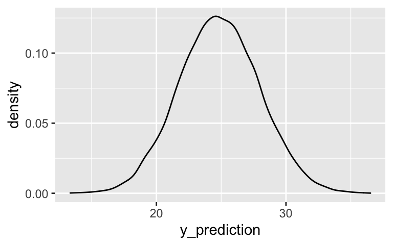

Posterior prediction: shortcut
They’re the same!

# Simulate a set of predictions
set.seed(84735)
shortcut_prediction <- posterior_predict(
    temp_posterior, newdata = data.frame(temp9am = 20))

# Construct a 90% posterior credible interval
posterior_interval(shortcut_prediction, prob = 0.9)
##         5%      95%
## 1 19.71731 30.02199

# Plot the approximate predictive model
mcmc_areas(shortcut_prediction, prob = 0.9) + 
  scale_x_continuous(breaks = seq(15, 35, by = 5)) + 
  xlab("3pm temperature")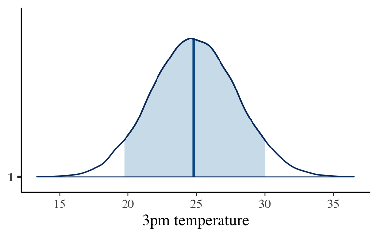

Posterior prediction follow-up

Using weakly informative priors

temp_prior_default <- stan_glm(
            temp3pm ~ temp9am, data = weather_perth,
            family = gaussian,
            prior_PD = TRUE,
            chains = 4, iter = 5000*2, seed = 84735, refresh = 0)

\(\beta_0 \sim N(24, 15^2)\), \(\beta_1 \sim N(0, 2.8^2)\), \(\sigma \sim Exp(0.17)\).

prior_summary(temp_prior_default)
## Priors for model 'temp_prior_default' 
## ------
## Intercept (after predictors centered)
##   Specified prior:
##     ~ normal(location = 24, scale = 2.5)
##   Adjusted prior:
##     ~ normal(location = 24, scale = 15)
## 
## Coefficients
##   Specified prior:
##     ~ normal(location = 0, scale = 2.5)
##   Adjusted prior:
##     ~ normal(location = 0, scale = 2.8)
## 
## Auxiliary (sigma)
##   Specified prior:
##     ~ exponential(rate = 1)
##   Adjusted prior:
##     ~ exponential(rate = 0.17)
## ------
## See help('prior_summary.stanreg') for more details

The Normal prior for \(\beta_1\) is centered at 0. Thus the default assumption is that the relationship between afternoon and morning temps might be positive, negative, or non-existent. This is a vague / weakly informative assumption.

The default priors are much more vague, but still on the general scale of temperatures (eg: not in the 1000s).

# Plot a prior predictive check
pp_check(temp_prior_default) +
  xlab("3pm temperature")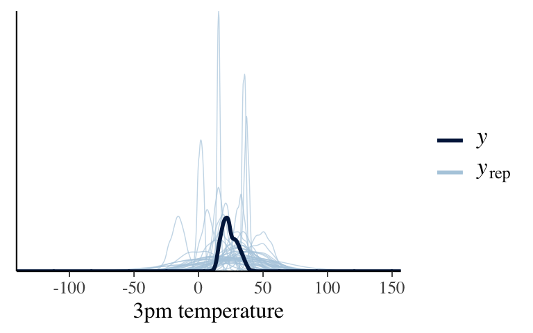


# 200 prior model lines
weather_perth %>%
  add_fitted_draws(temp_prior_default, n = 200) %>%
  ggplot(aes(x = temp9am, y = temp3pm)) +
    geom_line(aes(y = .value, group = .draw), alpha = 0.15)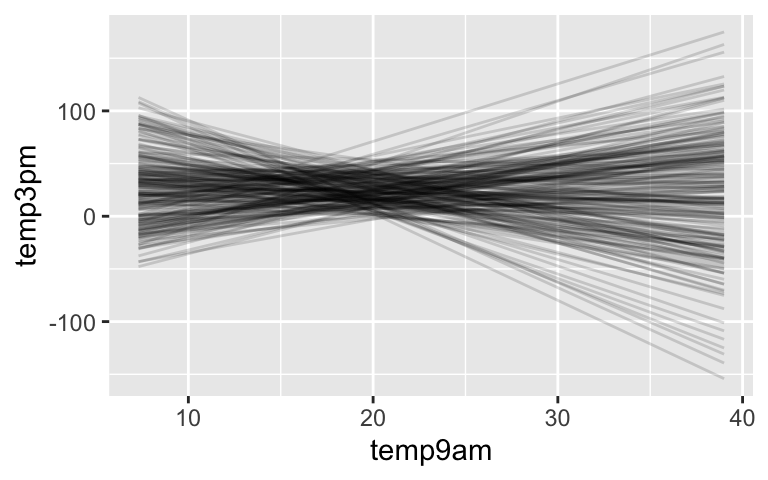


# Plot 4 prior simulated datasets
            weather_perth %>%
              add_predicted_draws(temp_prior_default, n = 4) %>%
              ggplot(aes(x = temp9am, y = temp3pm)) +
                geom_point(aes(y = .prediction, group = .draw), size = 0.1) +
                facet_wrap(~ .draw)