2 Bayes’ Rule: Thinking like a Bayesian

GOAL

Before jumping into Bayesian models, we need to start thinking like Bayesians.

RECOMMENDED READING

Bayes Rules! Chapters 1 and 2.

WHERE ARE WE?

2.1 Warm-up

Example 1

Imagine you were one of the lucky students to get into THDA 41, Modern Dance I.

1. Before the semester begins, what do you anticipate will be your final grade in the course?
   A+, A, A-, B+, B, B-, C+, C, C-

2. You earn an “A” on Homework 1. At this point, what do you anticipate will be your final grade in the course?
   A+, A, A-, B+, B, B-, C+, C, C-

3. You earn a “B” on Homework 2. At this point, what do you anticipate will be your final grade in the course?
   A+, A, A-, B+, B, B-, C+, C, C-

Example 2

Your roommate invites their childhood friend to stay with you for the weekend.

1. What’s the chance that you and your roommate’s friend will also become friends?

2. Your roommate’s friend arrived late last night. In the morning, before you meet them, you discover that they’ve eaten all of your cereal. At this point, what’s the chance that you and your roommate’s friend will also become friends?

BAYESIAN THINKING IS NATURAL

We naturally update our understanding of the world as new data come in. For example, in the warm-up, you considered your success in a dance course based on your prior experience with the subject and your first homework assignment. A Bayesian analysis uses a formal process to similarly conduct a more scientific inquiry, whether about voting patterns, climate change, public health, etc. No matter the scenario, you don’t walk into such an inquiry blind - you carry a degree of incoming information based on your prior research and experience. Naturally, it is in light of this incoming information that you interpret new data, weighing both in developing a set of updated information:

2.2 Exercises

To see how the Bayesian philosophy plays out in a data analysis, let’s build a simple email filter that classifies an incoming email as spam or non-spam based on the number of misspellings in a 5 word subject line. We’ll make the following assumptions based on a previous email collection:

• 10% of all incoming emails are spam;
• Among spam emails, each word in the subject line has a 25% chance of being misspelled. Among non-spam emails, this figure is lower at 5%.

Thus there are two RANDOM VARIABLES in this experiment:

\[\begin{split} Y & = \text{ the number of misspellings in the 5 word subject line} \\ \theta & = \text{ whether the email is spam or not (1 or 0)} \\ \end{split}\]

GOAL
Use the observed data on the subject line (\(Y\)) to guess whether the email is spam or not (\(\theta\)).

Background review

For two discrete variables \(Y\) and \(\theta\):
\[\begin{split} f(y) & = \text{ marginal behavior of $Y$} \\ f(y,\theta) & = \text{ joint behavior between $Y$ and $\theta$} \\ f(y|\theta) & = \text{ conditional dependence of $Y$ on $\theta$} \\ f(\theta|y) & = \text{ conditional dependence of $\theta$ on $Y$} \\ \end{split}\]

• By the Law of Total Probability we can specify \(f(y)\) using \(f(y|\theta)\) and \(f(\theta)\):

  \[f(y) = \sum_{\theta} f(y,\theta) = \sum_{\theta} f(\theta)f(y | \theta) \]

• By Bayes’ Rule we can specify \(f(\theta|y)\) using information about \(f(y)\), \(f(\theta)\), and \(f(y|\theta)\):

  \[f(\theta|y) = \frac{f(y,\theta)}{f(y)} = \frac{f(\theta)f(y | \theta)}{f(y)}\]

1. Intuition
   Without doing any formal calculations, in which of the following scenarios do you think you’d have enough evidence to classify the email as spam? In the 5-word subject line…

   • There are 0 misspelled words: “I’m your long lost cousin!”
   • There are 2 misspelled words: “Im your long lost cosin!”
   • There are 4 misspelled words: “Im yore lon lost cosin!”

   We’ll do this more formally below!

2. PRIOR: What do we understand about \(\theta\) before observing data \(Y\)?
   Before observing data on the email subject line (\(Y\)), we have some incoming or prior information about whether the email is spam (\(\theta\)). We can capture this information by the prior model of \(\theta\). Define the prior pmf \(f(\theta)\).

3. Conditional data model: How do the data \(Y\) depend upon \(\theta\)?
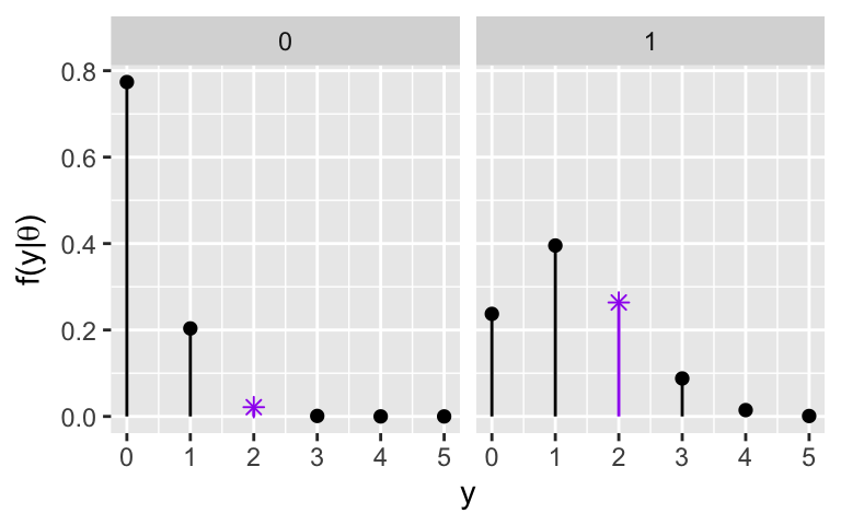
   To refine our understanding of \(\theta\), we can read the subject line and record \(Y\), the number of misspellings. \(Y\) is random and depends upon \(\theta\). This dependence is summarized by the conditional model of \(Y\) given \(\theta\).

   1. Define the conditional model, \(Y | \theta \; \sim \; ???\) and its corresponding pmf \(f(y| \theta) = P(Y=y|\theta)\).

   2. \(f(y|\theta)\) is plotted below. Summarize how the behavior of \(Y\) depends upon \(\theta\).

   

4. LIKELIHOOD FUNCTION: How compatible is our data with \(\theta\)?
   Now that we have some models set up, let’s observe some data. The next email you get has \(Y = 2\) misspellings. To process this data, we can flip how we think about the conditional pmf \(f(y|\theta)\). On its face, \(f(y|\theta)\) measures the probability of observing a yet unknown data point \(Y = y\) for a known given \(\theta\) value. Yet we find ourselves in the opposite situation: the observed data \(y\) is known and \(\theta\) (whether or not the email is spam) is unknown. To make this distinction, the likelihood function is defined by \(f(y|\theta)\) yet is a function of \(\theta\), not \(y\):

   \[L(\theta | y) := f(y | \theta)\]

   We can use this likelihood function of \(\theta\) to evaluate the relative likelihood or compatibility of our observed data \(Y=y\) with different possible \(\theta\).

   1. Summarize the likelihood function \(L(\theta| y=2)\) of \(\theta\) in the table below. Since this is a function of \(\theta\), not \(y\), it’s evaluated at all possible outcomes of \(\theta\) (here just 0 and 1).

      \(\theta\)	0	1	Total
      \(L(\theta | y = 2)\)	\(\hspace{1in}\)	\(\hspace{1in}\)	\(\hspace{1in}\)

   2. \(L(\theta| y=2)\) is plotted below. Convince yourself that this same information was staring us in the face in exercise 3, highlighted by asterisks. Essentially then, the likelihood function of \(\theta\) given the data that \(Y = 2\) extracts the information that matches this data from the conditional pmf \(f(y|\theta)\).

      

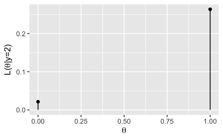
   3. According to the likelihood function, are the \(Y = 2\) misspellings more compatible with the email being spam or non-spam? Why?

   4. It’s important to note that a likelihood function \(L(\theta|y)\) is not a pmf for \(\theta\). Provide proof from the table in part a.

5. NORMALIZING CONSTANT: What’s the overall chance of observing data \(Y\)?
   The pmf \(f(y | \theta)\) summarizes the chances of getting \(Y = y\) misspelled words depending on whether the email is spam or non-spam (\(\theta\)). For frame of reference, what about the overall chance of observing \(Y=y\) across all emails (spam and non-spam combined), \(f(y)\)?

   1. Provide a formula for \(f(y)\).

   2. Use the formula from part a to calculate the probability that we would’ve observed \(Y = 2\) misspellings.

6. POSTERIOR: Bayes’ Rule
   The power of a Bayesian analysis is that it combines our prior information about \(\theta\) with the observed data to construct updated or posterior information about \(\theta\). In light of observing data \(Y=y\), the posterior model of \(\theta\) has pmf \(f(\theta | y)\). In this exercise, consider the posterior model in the general setting (not the email example).

   1. Use Bayes’ Rule to specify the general formula for constructing posterior pmf \(f(\theta|y)\) from the prior pmf \(f(\theta)\), likelihood function \(L(\theta|y)\), and normalizing constant \(f(y)\).

   2. In what scenarios will \(f(\theta|y)\) be small? That is, what has to be true about the prior and/or likelihood function of \(\theta\)? In what scenarios will \(f(\theta|y)\) be large?

7. POSTERIOR: What do we understand about \(\theta\) now that we’ve observed data \(Y\)?
   Back to our email.

   1. Specify the posterior pmf of the email’s spam status, \(\theta\), given we observed \(Y = 2\) misspellings.

      \(\theta\)	0	1	Total
      \(f(\theta | y = 2)\)	\(\hspace{1in}\)	\(\hspace{1in}\)	\(\hspace{1in}\)

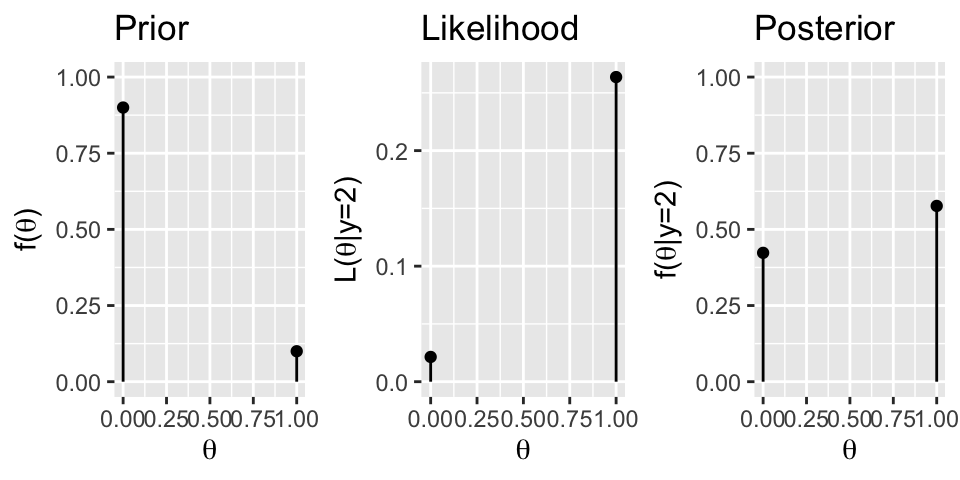
   2. The prior pmf, likelihood function, and posterior pmf of \(\theta\) are plotted below. Summarize the punchlines in the context of building a spam filter. (How does the posterior strike a balance between the prior and likelihood? Do you think our email is spam or not?)

      

8. Recommended: Extra practice
   Suppose that your next incoming email has \(Y = 1\) typos in the subject line. Define and interpret the posterior pmf \(f(\theta | y = 1)\).

9. Recommended: More extra practice
   Your friend has a bag with 3 dice: 2 are 4-sided and 1 is 6-sided. They pick a die at random, roll it once, and tell you the value.
   1. In this experiment, what’s our parameter \(\theta\)? What’s the data \(Y\)?
   2. Define the prior pmf \(f(\theta)\).
   3. Define the posterior pmf \(f(\theta | y)\) assuming your friend rolls \(Y = 5\).
   4. Define the posterior pmf \(f(\theta | y)\) assuming your friend rolls \(Y = 1\).

10. Optional: digging deeper
    For exercise 7, show that the posterior pmf \(f(\theta | y)\) can be calculated using the information from the prior \(f(\theta)\) and likelihood \(L(\theta|y)\) without calculating the normalizing constant \(f(y)\).

2.3 Bayes’ Rule

The power of a Bayesian analysis is that it combines our prior information about \(\theta\) with the observed data to construct updated or posterior information about \(\theta\):

Specifically, in light of observing data \(Y=y\), the posterior model of \(\theta\) has pmf

\[f(\theta | y) = \frac{f(\theta)L(\theta|y)}{f(y)}\]

where \(f(\theta|y)\) depends upon the following pieces:

• prior pmf
  \(f(\theta)\) reflects our prior information about \(\theta\)

• likelihood function
  \(L(\theta|y) := f(y|\theta)\) is a function of \(\theta\) that measures the relative likelihood of observing data \(Y = y\) for different possible values of \(\theta\). For example, if \(L(\theta_1|y) > L(\theta_2|y)\), then our data is more likely to have occurred if \(\theta = \theta_1\) than if \(\theta = \theta_2\). NOTE: The function \(L(\theta | y)\) is NOT a pmf for \(\theta\).

• normalizing constant
  \(f(y)\) measures the overall chance of observing \(Y=y\) across all possible values of \(\theta\), taking into account the prior plausibility of each possible \(\theta\). Specifically, by the Law of Total Probability: \[\begin{split} f(y) & = \sum_\theta f(y,\theta) = \sum_{\theta} f(y|\theta)f(\theta) = \sum_{\theta} L(\theta|y)f(\theta) \\ f(y) & = \int_\theta f(y,\theta)d\theta = \int_{\theta} f(y|\theta)f(\theta)d\theta = \int_{\theta} L(\theta|y)f(\theta)d\theta \\ \end{split}\]

  NOTE: We’ll see soon that \(f(y)\) merely serves as a normalizing constant which appropriately scales the posterior to sum / integrate to 1. Thus, we needn’t really calculate it!

2.4 Solutions

1. Intuition

2. PRIOR
   

   \(\theta\)	0	1	Total
   \(f(\theta)\)	0.9	0.1	1

3. Conditional data model

   1. \(Y | \theta \; \sim \; \text{Bin}(5, p)\) where \(p = 0.05\) when \(\theta=0\) and \(p = 0.25\) when \(\theta=1\). For \(y \in \{0,1,2,3,4,5\}\)
      \[f(y|\theta) = \begin{cases} \left(\begin{array}{c} 5 \\ y \end{array}\right) 0.05^y0.95^{5-y} & \theta = 0 \\ \left(\begin{array}{c} 5 \\ y \end{array}\right) 0.25^y 0.75^{5-y} & \theta = 1 \\ \end{cases}\]

   2. For non-spam, there would typically be 0 or 1 misspellings. For spam, the number of misspellings tends to be higher.

4. LIKELIHOOD FUNCTION

   1. .

      \(\theta\)	0	1	Total
      \(L(\theta | y = 2)\)	0.02143438	0.2636719	0.2851063

      For example,

      \[L(\theta=0|y=2) = f(y=2|\theta=0) = \left(\begin{array}{c} 5 \\ 2 \end{array}\right) 0.05^20.95^{5-2}\]

   2. .

   3. spam. \(L(\theta = 1 | y = 2) > L(\theta = 0 | y = 2)\)

   4. The likelihood sums to 0.2851063, not 1, across all values of \(\theta\).

5. NORMALIZING CONSTANT

   1. .
      \[f(y) = 0.9 \cdot \left(\begin{array}{c} 5 \\ y \end{array}\right) 0.05^y0.95^{5-y} + 0.1 \cdot\left(\begin{array}{c} 5 \\ y \end{array}\right) 0.25^y 0.75^{5-y} \;\; \text{ for } y \in \{0,1,2,3,4,5\}\]

   2. .
      \[f(y = 2) = 0.9 \cdot \left(\begin{array}{c} 5 \\ 2 \end{array}\right) 0.05^20.95^{5-2} + 0.1 \cdot\left(\begin{array}{c} 5 \\ 2 \end{array}\right) 0.25^2 0.75^{5-2} = 0.04565812\]

6. POSTERIOR: Bayes’ Rule

   1. \(f(\theta | y) = f(\theta)L(\theta |y ) / f(y)\)

   2. small: when either the prior plausibility of \(\theta\) is low or the data is incompatible with \(\theta\) (or both)

7. POSTERIOR

   1. .

      \(\theta\)	0	1	Total
      \(f(\theta | y = 3)\)	0.423	0.577	1

   2. We think the email is more likely to be spam now that we saw 2 misspellings. Further, the posterior is a balance between the prior and likelihood.

8. Recommended: Extra practice
   \[\begin{split} f(\theta) & = \begin{cases} 0.1 & \theta = 0 \\ 0.9 & \theta = 1 \\ \end{cases} \\ L(\theta | y = 1) & = \begin{cases} 0.2036266 & \theta = 0 \\ 0.3955078 & \theta = 1 \\ \end{cases} \\ f(y = 2) & = 0.9 \cdot \left(\begin{array}{c} 5 \\ 1 \end{array}\right) 0.05^10.95^{5-1} + 0.1 \cdot\left(\begin{array}{c} 5 \\ 1 \end{array}\right) 0.25^1 0.75^{5-1} = 0.2228147 \\ f(\theta | y = 2) & = \frac{f(\theta)L(\theta | y = 2)}{f(y=2)}\\ & = \begin{cases} 0.9*0.2036266/0.2228147 & \theta = 0 \\ 0.1*0.3955078/0.2228147 & \theta = 1 \\ \end{cases} \\ & = \begin{cases} 0.822 & \theta = 0 \\ 0.178 & \theta = 1 \\ \end{cases} \\ \end{split}\]

9. Recommended: More extra practice

   1. \(\theta\) is the number of sides the die has. \(Y\) is the value of the rolled die.

   2. .
      \[f(\theta) = \begin{cases} 2/3 & \theta = 4 \\ 1/3 & \theta = 6 \\ \end{cases}\]

   3. It’s impossible to roll \(Y=5\) if \(\theta = 4\), thus \[f(\theta|y = 5) = \begin{cases} 0 & \theta = 4 \\ 1 & \theta = 6 \\ \end{cases} \\\]

   4. .
      \[\begin{split} L(\theta|y = 1) & = \begin{cases} 1/4 & \theta = 4 \\ 1/6 & \theta = 6 \\ \end{cases} \\ f(y = 1) & = 2/3*1/4 + 1/3*1/6 = 2/ 9 \\ f(\theta|y = 1) & = f(\theta)L(\theta | y = 1) / f(y = 1) = \begin{cases} 3/4 & \theta = 4 \\ 1/4 & \theta = 6 \\ \end{cases} \\ \end{split}\]