11 Model evaluation & comparison
GOALS
In the context of Bayesian regression models of some response variable \(Y\) by predictor variables \(X\), we must be able to evaluate and compare different models. That is, we must ask:
- Is mine a good model?
- How do I choose between multiple possible models?
RECOMMENDED READING
Bayes Rules! Chapters 10 & 11.
11.1 Warm-up
We’ll continue to model 3pm temperatures (\(Y\)). This time, we’ll use various potential predictors and data on multiple locations: Uluru and Wollongong.
# Load packages
library(tidyverse)
library(tidybayes)
library(rstan)
library(rstanarm)
library(bayesplot)
library(bayesrules)
library(broom.mixed)

# Load data
weather <- read.csv("https://www.macalester.edu/~ajohns24/data/stat454/australia.csv")
Throughout, we’ll assume we have the following prior information:
The typical 3pm temperature on a typical day is likely around 30 degrees, but could be anywhere between 10 and 50 degrees (mean \(\pm\) 2 standard deviations).
Otherwise, we’ll assume we don’t have any prior information about the relationship between 3pm temperatures and other potential predictors, thus will utilize weakly informative priors.
Let’s start with a model of temp3pm (\(Y\)) vs temp9am (\(X_1\)):
\[\begin{split} Y_i | \beta_0, \beta_1, \sigma & \stackrel{ind}{\sim} N(\mu_i, \sigma^2) \;\; \text{ where } \mu_i = \beta_0 + \beta_1 X_{i1} \\ \beta_{0c} & \sim N(30, 10^2) \\ \beta_1 & \sim ... \\ \sigma & \sim ... \\ \end{split}\]
STEP 1: SIMULATE & UNDERSTAND THE PRIOR MODEL
# Simulate the prior model
model_1_prior <- stan_glm(
    temp3pm ~ temp9am, data = weather,
    family = gaussian,
    prior_intercept = normal(30, 10),
    prior_PD = TRUE,
    chains = 4, iter = 5000*2, seed = 84735, refresh = 0)

# Check out the prior tunings
prior_summary(model_1_prior)
## Priors for model 'model_1_prior'
## ------
## Intercept (after predictors centered)
##  ~ normal(location = 30, scale = 10)
##
## Coefficients
##   Specified prior:
##     ~ normal(location = 0, scale = 2.5)
##   Adjusted prior:
##     ~ normal(location = 0, scale = 3.1)
##
## Auxiliary (sigma)
##   Specified prior:
##     ~ exponential(rate = 1)
##   Adjusted prior:
##     ~ exponential(rate = 0.13)
## ------
## See help('prior_summary.stanreg') for more details

# Plot a prior predictive check
pp_check(model_1_prior) +
  xlab("temp3pm")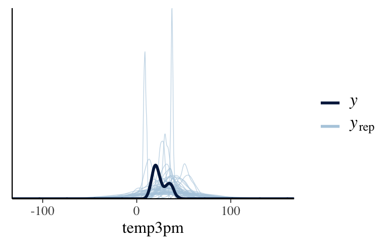
# 200 prior model lines
weather %>%
  add_fitted_draws(model_1_prior, n = 200) %>%
  ggplot(aes(x = temp9am, y = temp3pm)) +
    geom_line(aes(y = .value, group = .draw), alpha = 0.15)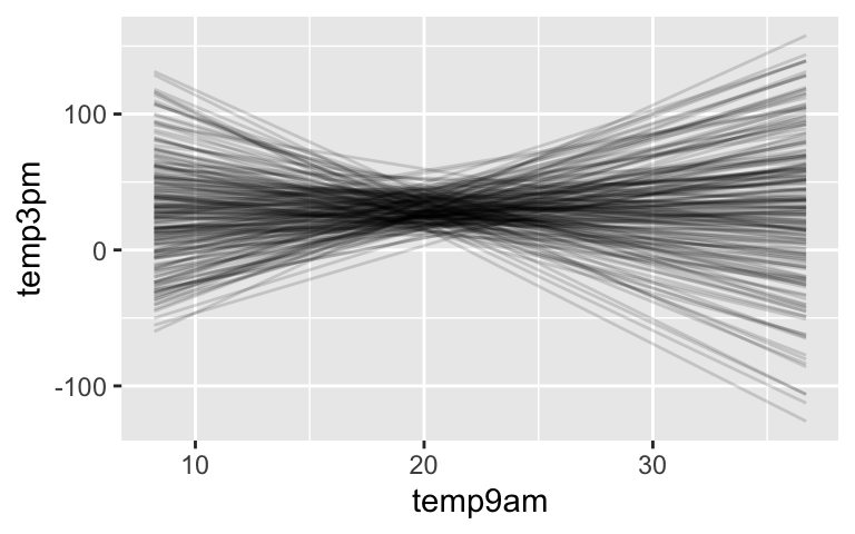
# Plot 4 prior simulated datasets
weather %>%
  add_predicted_draws(model_1_prior, n = 4) %>%
  ggplot(aes(x = temp9am, y = temp3pm)) +
    geom_point(aes(y = .prediction, group = .draw), size = 0.1) +
    facet_wrap(~ .draw)
STEP 2: CHECK OUT THE DATA
ggplot(weather, aes(x = temp9am, y = temp3pm)) +
    geom_point()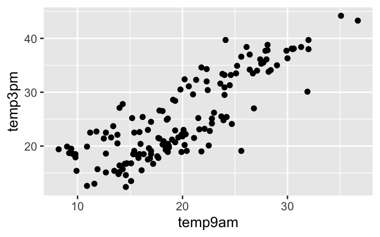
STEP 3: SIMULATE THE POSTERIOR
# Shortcut to simulating the posterior
model_1 <- update(model_1_prior, prior_PD = FALSE, refresh = 0)

## Or start from scratch
# model_1 <- stan_glm(
#   temp3pm ~ temp9am, data = weather,
#   family = gaussian,
#   prior_intercept = normal(30, 10),
#   chains = 4, iter = 5000*2, seed = 84735)
STEP 4: PERFORM MCMC DIAGNOSTICS
mcmc_trace(model_1)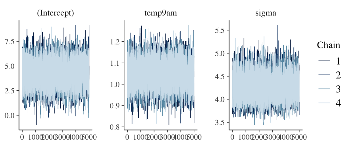
mcmc_dens_overlay(model_1)
STEP 5: ANALYZE THE POSTERIOR
tidy(model_1, effects = c("fixed", "aux"),
     conf.int = TRUE, conf.level = 0.80)
## # A tibble: 4 x 5
##   term        estimate std.error conf.low conf.high
##   <chr>          <dbl>     <dbl>    <dbl>     <dbl>
## 1 (Intercept)     4.26    1.18      2.75       5.79
## 2 temp9am         1.05    0.0573    0.973      1.12
## 3 sigma           4.26    0.252     3.96       4.60
## 4 mean_PPD       25.0     0.496    24.3       25.6
STEP 6: MODEL EVALUATION (& EVENTUAL SELECTION)
STEP 7: ITERATE & REPEAT!
Model building and evaluation is an iterative process. We build a model, evaluate it, “fix” it, build a new model, evaluate the new model, “fix” it, and so on. It’s nearly never the case that we build one model and call it quits.
11.2 Exercises
NOTE: So that your document will need before all chunks are complete, some chunks have eval = FALSE (meaning don’t evaluate this chunk when knitting). Once you have a chunk running, delete this or change it to eval = TRUE.
11.2.1 Model evaluation
- How fair is the model?
Answer this question in the context of our analysis. For example, think about the following:- How, by whom, and for what purpose was the data collected? Who was included in / excluded from this process?
- How might the results of the analysis, or the data collection itself, impact individuals and society?
- What biases might be baked into the analysis as a result of the data itself, our analysis of this data, or even our own perspectives?
How wrong is the model?
To answer this question, perform a posterior predictive check usingpp_check(). Does the underlying structure of our Normal regression model appear to be reasonable?pp_check(model_1)
- Fix the model
Thepp_check()revealed a structural issue with our model.- Identify what you think the issue is. Support your guess by constructing a relevant visualization of the raw weather data.
- Build and simulate a new model which fixes the issue. Store this as
model_2. NOTE: Do not taketemp9amout of the model and use the same priors. - Perform a
pp_check()to confirm thatmodel_2is structurally better thanmodel_1. - Chat with the instructor before moving on to ensure we’re all on the same page!
Visualize the new model
Don’t forget to deleteeval = FALSE!# NOTE: The same thing goes in both ___ weather %>% add_fitted_draws(model_2, n = 200) %>% ggplot(aes(x = temp9am, y = temp3pm, color = ___)) + geom_line(aes(y = .value, group = paste(___, .draw)), alpha = 0.15) + geom_point(data = weather)
- How accurate are the posterior predictions?
We can assess the quality of predictions using both visual and numerical summaries.Plot the posterior predictive models for all data points:
# First obtain posterior predictive models
# for each data point in weather:
set.seed(84735)
predictions_2 <- posterior_predict(model_2, newdata = weather)

# Plot the posterior predictive intervals
ppc_intervals_grouped(
  weather$temp3pm, yrep = predictions_2,
  x = weather$temp9am, group = weather$location,
  prob = 0.5, prob_outer = 0.95,
  facet_args = list(scales = "fixed")) +
  labs(x = "temp9am", y = "temp3pm")
Evaluate the accuracy of the posterior predictions. Interpret each of the four reported numbers and make sure you can match them to the plot in part a.
set.seed(84735)
prediction_summary(model = model_2, data = weather)
New data!
Next, suppose we want to use this model to predicttemp3pmfor 50 new days:new_data <- read.csv("https://www.macalester.edu/~ajohns24/data/stat454/australia_2.csv")- Do you think our new model will be as accurate in predicting
temp3pmfor these new days as it was for the days in our original sample? Explain.
- Try it out. Evaluate the accuracy of our model’s posterior predictions for the
new_data.
- Do you think our new model will be as accurate in predicting
Cross-validation
The previous exercise provides a warning: our model is optimized to our sample data, thus will tend to be better at predicting this sample data than new data points. It’s then more responsible to evaluate our model’s posterior predictive accuracy when applied to new data. In practice, we only have 1 data set, not 2 (i.e. we don’t havenew_datato play with). Cross-validation allows us to both build our model using this data and evaluate how well it might perform on new data. You’ll learn about the details for the next class. For now, apply the cross-validation technique:# (Bad) approach 1: # Evaluate accuracy in predicting the same data we used to build the model set.seed(84735) prediction_summary(model = model_2, data = weather) # (Better) approach 2: # Evaluate accuracy in predicting the NEW data set.seed(84735) prediction_summary_cv(model = model_2, data = weather, k = 10)$cv- In terms of MAE, how accurate is our model at predicting the
temp3pmvalues in our original sample? - In terms of MAE, how accurate is our model at predicting
temp3pmvalues on NEW days? - When communicating the posterior prediction accuracy for our model, which number should you report?
- In terms of MAE, how accurate is our model at predicting the
- Is my model good vs is my Markov chain simulation good?
We’ve now learned how to evaluate our Bayesian posterior models, and how to perform diagnostics for evaluating the quality of our Markov chain simulation. What’s the difference between these two goals?
11.2.2 Model comparison
Using a sample of data on just Wollongong, let’s model temp3pm (\(Y\)) by day_of_year, 1 through 365 (\(X\)):
# Obtain the sample data
wollongong <- read.csv("https://www.macalester.edu/~ajohns24/data/stat454/weather_sample_1.csv")

# Plot temp3pm vs day_of_year
ggplot(wollongong, aes(x = day_of_year, y = temp3pm)) +
  geom_point()
Consider 3 polynomial models of this relationship:
mod_1has 0 predictors: \[\mu = \beta_0\]mod_2assumes a quadratic relationship, thus has 2 predictors: \[\mu = \beta_0 + \beta_1 X + \beta_2 X^2\]mod_3assumes a 12th order polynomial relationship, thus has 12 predictors: \[\mu = \beta_0 + \beta_1 X + \beta_2 X^2 + \cdots + \beta_{12} X^{12}\]
Simulate the posteriors for these models:
mod_1 <- stan_glm(
    temp3pm ~ 1, data = wollongong,
    family = gaussian,
    prior_intercept = normal(30, 10),
    chains = 4, iter = 5000*2, seed = 84735, refresh = 0)

mod_2 <- stan_glm(
    temp3pm ~ poly(day_of_year, 2), data = wollongong,
    family = gaussian,
    prior_intercept = normal(30, 10),
    chains = 4, iter = 5000*2, seed = 84735, refresh = 0)

mod_3 <- stan_glm(
    temp3pm ~ poly(day_of_year, 12), data = wollongong,
    family = gaussian,
    prior_intercept = normal(30, 10),
    chains = 4, iter = 5000*2, seed = 84735, refresh = 0)
Plot 200 posterior model lines / curves for each model:
wollongong %>%
  add_fitted_draws(mod_1, n = 200) %>%
  ggplot(aes(x = day_of_year, y = temp3pm)) +
    geom_line(aes(y = .value, group = .draw), alpha = 0.15) +
    geom_point(data = wollongong)

wollongong %>%
  add_fitted_draws(mod_2, n = 200) %>%
  ggplot(aes(x = day_of_year, y = temp3pm)) +
    geom_line(aes(y = .value, group = .draw), alpha = 0.15) +
    geom_point(data = wollongong)

wollongong %>%
  add_fitted_draws(mod_3, n = 200) %>%
  ggplot(aes(x = day_of_year, y = temp3pm)) +
    geom_line(aes(y = .value, group = .draw), alpha = 0.15) +
    geom_point(data = wollongong)
- Which is the best model?
- Examine the
pp_check()for each model. Which model is the most wrong? The least? - Which model do you think will have the best “in-sample” prediction error, that is the best predictions of the data points in our
wollongongsample? Test your guess with aprediction_summary()of each model. - Which model do you think will have the best cross-validated prediction error, that is the best predictions of new data points? Test your guess with a
prediction_summary_cv()$cvof each model.
- Examine the
Overfitting & the bias-variance trade-off
The reason thatmod_3performed so poorly when applied to new data is that it was overfit to our sample data. That is, it did a great job of detecting the specific details in our data, to the detriment of its applicability to new data. In general, in modeling, we’re looking for a model that wins the bias-variance trade-off. To explore this idea, run the animation below which plots our 3 models for each of 20 different possible data sets. Then answer the follow-up questions.library(infer) library(gganimate) # Simulate 20 potential data sets of 40 days each twenty_data_sets <- wollongong %>% rep_sample_n(size = 40, replace = TRUE, reps = 5) %>% slice(rep(row_number(), 3)) %>% ungroup() %>% mutate(order = rep(rep(c(0,2,12), each = 40), 5)) # Construct an animated plot animated_plot <- ggplot(twenty_data_sets, aes(x = day_of_year, y = temp3pm)) + geom_point() + facet_wrap(~ order) + stat_smooth(data = twenty_data_sets %>% filter(order == 0), formula = y ~ 1, method = "lm", se = FALSE) + stat_smooth(data = twenty_data_sets %>% filter(order == 2), formula = y ~ poly(x,2), method = "lm", se = FALSE) + stat_smooth(data = twenty_data_sets %>% filter(order == 12), formula = y ~ poly(x,12), method = "lm", se = FALSE) + ylim(12, 27) + transition_states(replicate, transition_length = 0, state_length = 1) # Now animate that plot! animate(animated_plot, fps = 20)- Which model tends to vary the most from sample to sample? The least?
- Which model tends to be the closest to the sample data points, i.e. has the least bias? The most bias?
- We want a model that maintains low bias and low variance. Which model does so?
11.3 Solutions
- How fair is the model?
How wrong is the model?
It’s wrong. The data is bi-modal but our simulated 3pm temps are not.pp_check(model_1)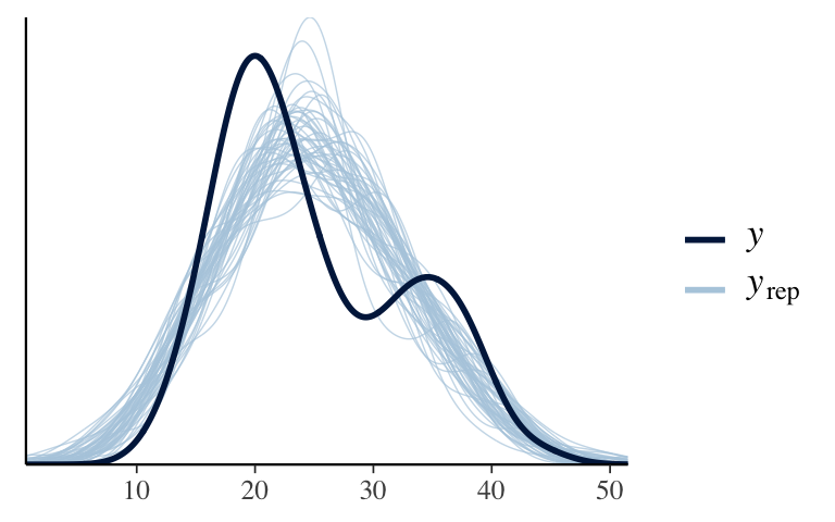
Fix the model
# a. The bimodality is explained by location ggplot(weather, aes(x = temp3pm, color = location)) + geom_density()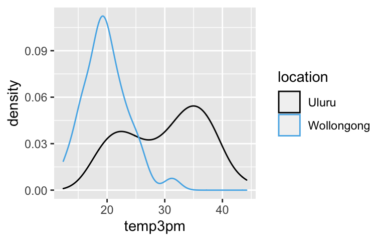
# b. Add location as a predictor. model_2 <- stan_glm( temp3pm ~ temp9am + location, data = weather, family = gaussian, prior_intercept = normal(30, 10), chains = 4, iter = 5000*2, seed = 84735) ## ## SAMPLING FOR MODEL 'continuous' NOW (CHAIN 1). ## Chain 1: ## Chain 1: Gradient evaluation took 1.9e-05 seconds ## Chain 1: 1000 transitions using 10 leapfrog steps per transition would take 0.19 seconds. ## Chain 1: Adjust your expectations accordingly! ## Chain 1: ## Chain 1: ## Chain 1: Iteration: 1 / 10000 [ 0%] (Warmup) ## Chain 1: Iteration: 1000 / 10000 [ 10%] (Warmup) ## Chain 1: Iteration: 2000 / 10000 [ 20%] (Warmup) ## Chain 1: Iteration: 3000 / 10000 [ 30%] (Warmup) ## Chain 1: Iteration: 4000 / 10000 [ 40%] (Warmup) ## Chain 1: Iteration: 5000 / 10000 [ 50%] (Warmup) ## Chain 1: Iteration: 5001 / 10000 [ 50%] (Sampling) ## Chain 1: Iteration: 6000 / 10000 [ 60%] (Sampling) ## Chain 1: Iteration: 7000 / 10000 [ 70%] (Sampling) ## Chain 1: Iteration: 8000 / 10000 [ 80%] (Sampling) ## Chain 1: Iteration: 9000 / 10000 [ 90%] (Sampling) ## Chain 1: Iteration: 10000 / 10000 [100%] (Sampling) ## Chain 1: ## Chain 1: Elapsed Time: 0.159733 seconds (Warm-up) ## Chain 1: 0.203732 seconds (Sampling) ## Chain 1: 0.363465 seconds (Total) ## Chain 1: ## ## SAMPLING FOR MODEL 'continuous' NOW (CHAIN 2). ## Chain 2: ## Chain 2: Gradient evaluation took 1.8e-05 seconds ## Chain 2: 1000 transitions using 10 leapfrog steps per transition would take 0.18 seconds. ## Chain 2: Adjust your expectations accordingly! ## Chain 2: ## Chain 2: ## Chain 2: Iteration: 1 / 10000 [ 0%] (Warmup) ## Chain 2: Iteration: 1000 / 10000 [ 10%] (Warmup) ## Chain 2: Iteration: 2000 / 10000 [ 20%] (Warmup) ## Chain 2: Iteration: 3000 / 10000 [ 30%] (Warmup) ## Chain 2: Iteration: 4000 / 10000 [ 40%] (Warmup) ## Chain 2: Iteration: 5000 / 10000 [ 50%] (Warmup) ## Chain 2: Iteration: 5001 / 10000 [ 50%] (Sampling) ## Chain 2: Iteration: 6000 / 10000 [ 60%] (Sampling) ## Chain 2: Iteration: 7000 / 10000 [ 70%] (Sampling) ## Chain 2: Iteration: 8000 / 10000 [ 80%] (Sampling) ## Chain 2: Iteration: 9000 / 10000 [ 90%] (Sampling) ## Chain 2: Iteration: 10000 / 10000 [100%] (Sampling) ## Chain 2: ## Chain 2: Elapsed Time: 0.138572 seconds (Warm-up) ## Chain 2: 0.233279 seconds (Sampling) ## Chain 2: 0.371851 seconds (Total) ## Chain 2: ## ## SAMPLING FOR MODEL 'continuous' NOW (CHAIN 3). ## Chain 3: ## Chain 3: Gradient evaluation took 2e-05 seconds ## Chain 3: 1000 transitions using 10 leapfrog steps per transition would take 0.2 seconds. ## Chain 3: Adjust your expectations accordingly! ## Chain 3: ## Chain 3: ## Chain 3: Iteration: 1 / 10000 [ 0%] (Warmup) ## Chain 3: Iteration: 1000 / 10000 [ 10%] (Warmup) ## Chain 3: Iteration: 2000 / 10000 [ 20%] (Warmup) ## Chain 3: Iteration: 3000 / 10000 [ 30%] (Warmup) ## Chain 3: Iteration: 4000 / 10000 [ 40%] (Warmup) ## Chain 3: Iteration: 5000 / 10000 [ 50%] (Warmup) ## Chain 3: Iteration: 5001 / 10000 [ 50%] (Sampling) ## Chain 3: Iteration: 6000 / 10000 [ 60%] (Sampling) ## Chain 3: Iteration: 7000 / 10000 [ 70%] (Sampling) ## Chain 3: Iteration: 8000 / 10000 [ 80%] (Sampling) ## Chain 3: Iteration: 9000 / 10000 [ 90%] (Sampling) ## Chain 3: Iteration: 10000 / 10000 [100%] (Sampling) ## Chain 3: ## Chain 3: Elapsed Time: 0.149162 seconds (Warm-up) ## Chain 3: 0.241485 seconds (Sampling) ## Chain 3: 0.390647 seconds (Total) ## Chain 3: ## ## SAMPLING FOR MODEL 'continuous' NOW (CHAIN 4). ## Chain 4: ## Chain 4: Gradient evaluation took 2e-05 seconds ## Chain 4: 1000 transitions using 10 leapfrog steps per transition would take 0.2 seconds. ## Chain 4: Adjust your expectations accordingly! ## Chain 4: ## Chain 4: ## Chain 4: Iteration: 1 / 10000 [ 0%] (Warmup) ## Chain 4: Iteration: 1000 / 10000 [ 10%] (Warmup) ## Chain 4: Iteration: 2000 / 10000 [ 20%] (Warmup) ## Chain 4: Iteration: 3000 / 10000 [ 30%] (Warmup) ## Chain 4: Iteration: 4000 / 10000 [ 40%] (Warmup) ## Chain 4: Iteration: 5000 / 10000 [ 50%] (Warmup) ## Chain 4: Iteration: 5001 / 10000 [ 50%] (Sampling) ## Chain 4: Iteration: 6000 / 10000 [ 60%] (Sampling) ## Chain 4: Iteration: 7000 / 10000 [ 70%] (Sampling) ## Chain 4: Iteration: 8000 / 10000 [ 80%] (Sampling) ## Chain 4: Iteration: 9000 / 10000 [ 90%] (Sampling) ## Chain 4: Iteration: 10000 / 10000 [100%] (Sampling) ## Chain 4: ## Chain 4: Elapsed Time: 0.189711 seconds (Warm-up) ## Chain 4: 0.232731 seconds (Sampling) ## Chain 4: 0.422442 seconds (Total) ## Chain 4: # c. pp_check(model_2)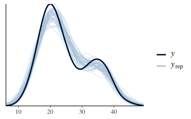
Visualize the new model
# NOTE: The same thing goes in both ___ weather %>% add_fitted_draws(model_2, n = 200) %>% ggplot(aes(x = temp9am, y = temp3pm, color = location)) + geom_line(aes(y = .value, group = paste(location, .draw)), alpha = 0.15) + geom_point(data = weather)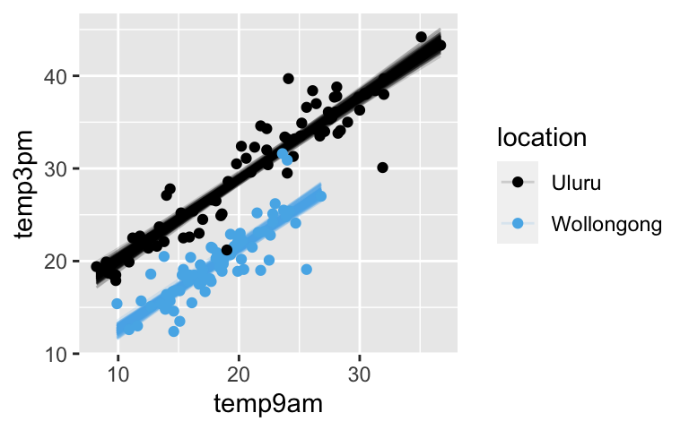
- How accurate are the posterior predictions?
.
# First obtain posterior predictive models # for each data point in weather: set.seed(84735) predictions_2 <- posterior_predict(model_2, newdata = weather) # Plot the posterior predictive intervals ppc_intervals_grouped( weather$temp3pm, yrep = predictions_2, x = weather$temp9am, group = weather$location, prob = 0.5, prob_outer = 0.95, facet_args = list(scales = "fixed")) + labs(x = "temp9am", y = "temp3pm")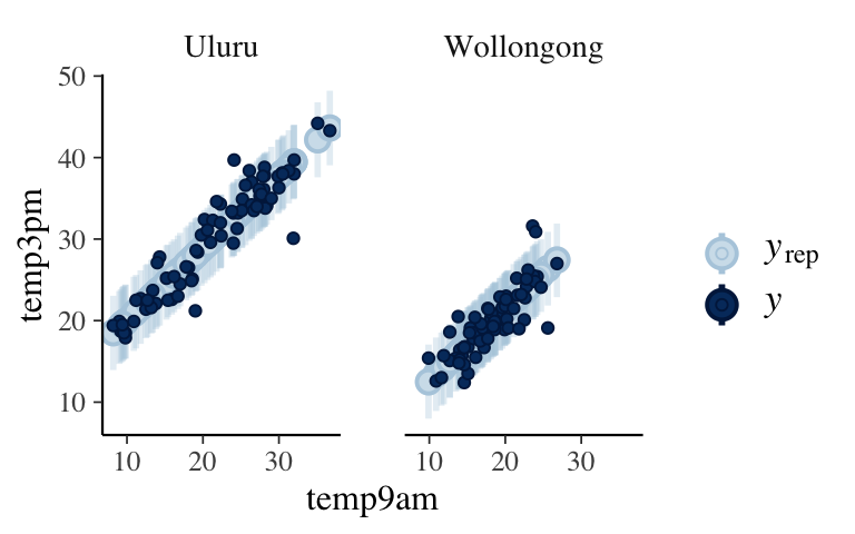
Observed temps are typically 1.07 degrees (0.47 standard deviations) from their posterior predictive means. On the scale of temperatures, this is quite accurate! Further, 65% are within their 50% prediction intervals (hence fall close to the posterior mean) and 95% within their 95% prediction intervals.
set.seed(84735) prediction_summary(model = model_2, data = weather)
New data!
new_data <- read.csv("https://www.macalester.edu/~ajohns24/data/stat454/australia_2.csv")Answers will vary.
The MAE and scaled MAE are bigger / worse.
set.seed(84735) prediction_summary(model = model_2, data = new_data) ## mae mae_scaled within_50 within_95 ## 1 1.212335 0.5306616 0.64 0.96
Cross-validation
# (Bad) approach 1: # Evaluate accuracy in predicting the same data we used to build the model set.seed(84735) prediction_summary(model = model_2, data = weather) ## mae mae_scaled within_50 within_95 ## 1 1.07095 0.4715991 0.6466667 0.9533333 # (Better) approach 2: # Evaluate accuracy in predicting the NEW data set.seed(84735) prediction_summary_cv(model = model_2, data = weather, k = 10)$cv ## mae mae_scaled within_50 within_95 ## 1 1.197039 0.5258567 0.6333333 0.94- posterior predictive means tend to be 1.07 degrees from the observed values
- posterior predictive means tend to be 1.197 degrees from the new values
- the cross-validated metric is more “fair” or conservative and also better captures how well our model might generalize outside our particular sample data
- Is my model good vs is my Markov chain simulation good?
- Is my model good: this evaluates the quality of our Bayesian model.
- Is my Markov chain simulation good: this evaluates our approximation of the Bayesian model.
- Ideally, both are good. But it’s possible to have a bad approximation of a good model, or a good approximation of a bad model, or a bad approximation of a bad model.
g1 <- wollongong %>%
add_fitted_draws(mod_1, n = 200) %>%
ggplot(aes(x = day_of_year, y = temp3pm)) +
geom_line(aes(y = .value, group = .draw), alpha = 0.15) +
geom_point(data = wollongong)
g2 <- wollongong %>%
add_fitted_draws(mod_2, n = 200) %>%
ggplot(aes(x = day_of_year, y = temp3pm)) +
geom_line(aes(y = .value, group = .draw), alpha = 0.15) +
geom_point(data = wollongong)
g3 <- wollongong %>%
add_fitted_draws(mod_3, n = 200) %>%
ggplot(aes(x = day_of_year, y = temp3pm)) +
geom_line(aes(y = .value, group = .draw), alpha = 0.15) +
geom_point(data = wollongong)
grid.arrange(g1, g2, g3, ncol=3)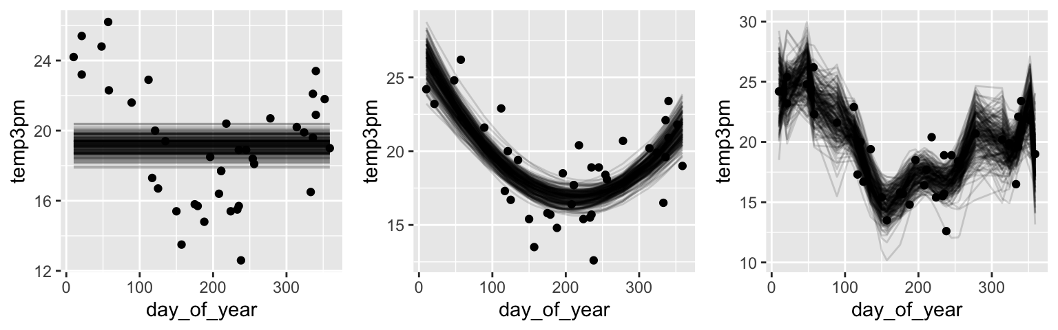
- Which is the best model?
most wrong = 1. least wrong = 2 / 3
mod_3has the best “in-sample” prediction errors:set.seed(84735) prediction_summary(mod_1, data = wollongong) ## mae mae_scaled within_50 within_95 ## 1 2.665252 0.7652436 0.425 0.975 prediction_summary(mod_2, data = wollongong) ## mae mae_scaled within_50 within_95 ## 1 1.544089 0.6755007 0.5 1 prediction_summary(mod_3, data = wollongong) ## mae mae_scaled within_50 within_95 ## 1 1.02678 0.4337498 0.65 1mod_2has the best predictions of new data points:set.seed(84735) prediction_summary_cv(model = mod_1, data = wollongong, k = 10)$cv ## mae mae_scaled within_50 within_95 ## 1 2.731204 0.7903701 0.425 0.975 prediction_summary_cv(model = mod_2, data = wollongong, k = 10)$cv ## mae mae_scaled within_50 within_95 ## 1 1.669499 0.716508 0.5 0.975 prediction_summary_cv(model = mod_3, data = wollongong, k = 10)$cv ## mae mae_scaled within_50 within_95 ## 1 1.98013 0.7010192 0.425 0.975
Overfitting & the bias-variance trade-off
library(infer) library(gganimate) # Simulate 20 potential data sets of 40 days each twenty_data_sets <- wollongong %>% rep_sample_n(size = 40, replace = TRUE, reps = 5) %>% slice(rep(row_number(), 3)) %>% ungroup() %>% mutate(order = rep(rep(c(0,2,12), each = 40), 5)) # Construct an animated plot animated_plot <- ggplot(twenty_data_sets, aes(x = day_of_year, y = temp3pm)) + geom_point() + facet_wrap(~ order) + stat_smooth(data = twenty_data_sets %>% filter(order == 0), formula = y ~ 1, method = "lm", se = FALSE) + stat_smooth(data = twenty_data_sets %>% filter(order == 2), formula = y ~ poly(x,2), method = "lm", se = FALSE) + stat_smooth(data = twenty_data_sets %>% filter(order == 12), formula = y ~ poly(x,12), method = "lm", se = FALSE) + ylim(12, 27) + transition_states(replicate, transition_length = 0, state_length = 1) # Now animate that plot! animate(animated_plot, fps = 20)mod_3varies the most, andmod_1the leastmod_3tends to be the least biased andmod_1the mostmod_2