6 Simulation: MCMC with rstan
GOALS
Use Monte Carlo and Markov chain Monte Carlo (MCMC) techniques to approximate posterior models. For the latter, we’ll utilize the
rstanpackage.Explore MCMC diagnostic tools that can help us answer “is this a good simulation?”
RECOMMENDED READING
Bayes Rules! Chapter 6.
6.1 R code reference
In the code below:
my_simis astanfitobject created using thestan()function- the
parsargument is completed by the label for our parameter of interest (eg:piorlambdaor…)
# Load packages
library(tidyverse)
library(rstan)
library(rstanarm)
library(bayesplot)
library(bayesrules)

# Density plot and histogram of the combined chain values
# pars is the name of the parameter we'd like to plot (eg: pi)
mcmc_dens(my_sim, pars = "___") +
  yaxis_text(TRUE) +
  ylab("density")

mcmc_hist(my_sim, pars = "___") +
  yaxis_text(TRUE) +
  ylab("count")


# Visual diagnostics: trace plots
mcmc_trace(my_sim, pars = "___", size = 0.5)
mcmc_trace(my_sim, pars = "___", size = 0.5, window = c(0, ___))  # This zooms in


# Visual diagnostics: overlaid density plots for all parallel chains
mcmc_dens_overlay(my_sim, pars = "___")


# Visual diagnostics: autocorrelation plots
mcmc_acf(my_sim, pars = "___")


# Numerical diagnostics: R-hat and effective sample size ratio
rhat(my_sim, pars = "___")
neff_ratio(my_sim, pars = "___")
6.2 Exercises
Let \(\pi\) be some proportion of interest (eg: your MCSG election support) and \(Y\) be the number of successes in 10 independent trials, each with probability of success \(\pi\). Consider the following Beta-Binomial model:
\[\begin{split} Y | \pi & \sim \text{Bin}(10, \pi) \\ \pi & \sim \text{Beta}(2, 2) \\ \end{split}\]
Further, suppose we observe \(Y = 9\) successes. Then the posterior model of \(\pi\) is
\[\pi | (Y=9) \sim \text{Beta}(11, 3)\]
Throughout the remainder of the activity, we’ll try to approximate this posterior using simulation techniques.
# Load some packages
library(tidyverse)
library(rstan)
library(rstanarm)
library(bayesplot)
library(bayesrules)
Monte Carlo drawbacks
We could approximate the Beta-Binomial posterior using the same Monte Carlo method from Homework 2:# Simulate the sample set.seed(454) mc_sample <- data.frame(pi = rbeta(100000, 2, 2)) %>% # Simulate pi from prior mutate(y = rbinom(100000, size = 10, prob = pi)) %>% # Simulate y from pi filter(y == 9) # Keep pi values that match our data # Use the sample to approximate the posterior ggplot(mc_sample, aes(x = pi)) + geom_density() + stat_function(fun = dbeta, args = list(shape1 = 11, shape2 = 3), color = "red")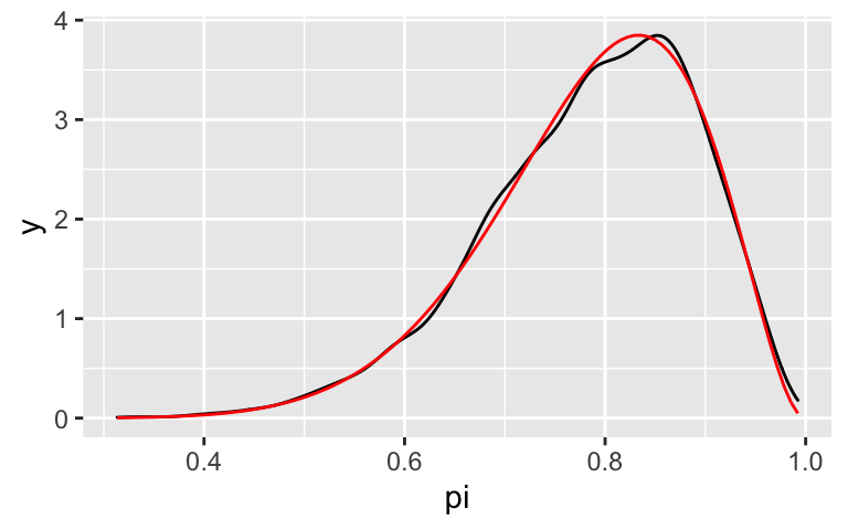
This Monte Carlo strategy works here, but has serious drawbacks / limitations. (There are other strategies, but they too have their unique limitations!)
- For what Beta-Binomial settings do you think this Monte Carlo method would fail to produce an accurate approximation? (What steps of this process won’t scale up?) Prove your point by changing the code above.
- Explain why we couldn’t use this same technique to simulate Bayesian models with continuous data \(Y\), such as the Normal-Normal.
MCMC with rstan
MCMC methods are more flexible and scale up to more complicated models. In this exercise, you’ll use therstanpackage to run an MCMC simulation for the Beta-Binomial model. You’re given all the syntax you need, and learned about this syntax in a video you watched for today.# STEP 1: Define the Beta-Binomial model in rstan notation bb_model <- " data { real<lower=0> alpha; real<lower=0> beta; int<lower=1> n; int<lower=0, upper=n> Y; } parameters { real<lower=0, upper=1> pi; } model { Y ~ binomial(n, pi); pi ~ beta(alpha, beta); } " # STEP 2: Simulate the posterior set.seed(84735) # Set the random number seed bb_sim <- stan( model_code = bb_model, data = list(alpha = 2, beta = 2, Y = 9, n = 10), chains = 4, iter = 10000*2)NOTE: If you get any errors and can’t run the above code, you can import the simulation results.
bb_sim <- readRDS(url("https://www.macalester.edu/~ajohns24/data/stat454/bb_sim.rds"))
Object structure
Examine the class and structure of thebb_simobject.# Check out what's stored in bb_sim # NOTE: lp__ is a scaled log likelihood function. We'll ignore it. bb_sim %>% names() # Check out the dimensions as.array(bb_sim, pars = "pi") %>% dim() # Check out the chains as.array(bb_sim, pars = "pi") %>% head()- How many chains did we run?
- We ran each chain for 20,000 iterations. By default, the first portion of chain values are thrown out as “burn-in” or “warm-up” samples, the idea being that it takes some time before a Markov chain starts producing values that mimic a random sample from the posterior. (Kind of like the first pancake in the batch is typically sub-par.) What proportion of chain values are tossed out?
- Combining all chains, what’s our total Markov chain sample size?
- Density plots & histograms: distribution of chain values
The distribution of the combined 40,000 chain values approximates the Bayesian posterior model. To check out the approximation, construct a density plot and histogram of the combined chain values. NOTE: Use
pars = "pi".In this illustrative example, we know the posterior is a Beta(11,3) and thus can compare it to our approximation. How did we do?
#mcmc_dens(___, ___) + # stat_function(fun = dbeta, args = list(11, 3), color = "red")
- Visual diagnostics: trace plots
In practice, we won’t know the posterior, thus won’t be able to assess the quality of our MCMC approximation by comparing it to the posterior. Instead, we can assess the quality of our chain using a variety of visual and numerical diagnostics. For visual diagnostics, trace plots illustrate the longitudinal behavior of a Markov chain, ie. the sequence in which we observed our chain values.- Construct trace plots of all 4 chains.
- Construct another set of trace plots that zooms in on the first 100 steps / iterations.
- Summarize what you observe.
Visual diagnostics: trace plots continued
To better understand if our trace plots are “good” or “bad,” consider some examples. Below are trace plots (left) and density plots (right) for three hypothetical Markov chain simulations: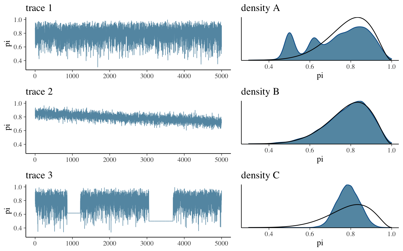
- Match each trace plot to its corresponding density plot.
- Based on these observations, summarize the features of a “good” trace plot.
- Summarize two possible features of a “bad” trace plot and the corresponding consequences on our posterior approximation.
- Based on these observations, are the trace plots for our
bb_simgood or bad?
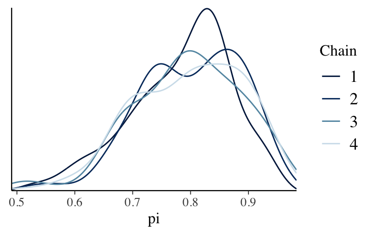
- Visual diagnostics: Comparing parallel chains
Run a new shorter simulation, with 4 parallel chains that each have 100 iterations after tossing out the burn-in.
# Set the random number seed set.seed(84735) # Simulate the posterior #bb_sim_short <- stan( # model_code = ___, # data = list(alpha = 2, beta = 2, Y = 9, n = 10), # chains = ___, iter = ___)NOTE: If you get any errors and can’t run the above code, you can import the simulation results.
bb_sim_short <- readRDS(url("https://www.macalester.edu/~ajohns24/data/stat454/bb_sim_short.rds"))For both
bb_simandbb_sim_short, check out density plots of the 4 parallel chains (not of all chain values combined). Use these plots to explain why running parallel chains can help us diagnose the quality of an MCMC simulation and what, ideally, we’d see in these plots.
- Recommended: Take note
Being respectful to your future self, take a few minutes to summarize the punchlines from today’s activity.
Recommended: More practice
Try to generalize thebb_modelsyntax: run astan()MCMC simulation of the posterior from the following Bayesian model upon the observation that \(Y = 20\). Summarize your simulation using plots, and perform a set of diagnostics.\[\begin{split} Y|\lambda & \sim Pois(\lambda) \\ \lambda & \sim Gamma(1,2) \\ \end{split}\]
- Optional: Another visual diagnostic – autocorrelation plots
By the construction of a Markov chain, chain values are inherently correlated – one chain value depends upon the previous chain value, which depends upon the one before that, which depends upon the one before that, and so on. This also means that each chain value depends in some degree on all previous chain values. Yet this dependence, or autocorrelation, fades. Specifically, it’s typically the case that the lag 1 autocorrelation between two subsequent chain values (eg: \(\pi^{(100)}\) and \(\pi^{(99)}\)) is bigger than the lag 10 autocorrelation between two chain values that are 10 steps apart (eg: \(\pi^{(100)}\) and \(\pi^{(90)}\)).- What do you think is more advantageous, autocorrelation among chain values which fades quickly or fades slowly? Why?
- Construct and comment on autocorrelation plots for your simulation. Based on this diagnostic, is our simulation good or bad?
- Optional: Numerical diagnostics
Visual diagnostics aren’t perfect and can get tedious when we have bigger models. Thus it can help to supplement visual diagnostics with numerical diagnostics. Two examples are the “R-hat” and the “effective sample size ratio” metrics. R-hat reflects the degree of discrepancy in our parallel chains (the greater the discrepancy the worse our simulation), thus is a numerical complement to comparing trace and density plots for our parallel chains. Effective sample size ratios measure the degree to which the autocorrelation in our chains decreases the effectiveness of our simulation relative to taking a hypothetical random sample from the posterior, thus is a numerical complement to the autocorrelation plot. If you’re curious, read 6.3.3 and 6.3.4. Using the code there, calculate and interpret R-hat and the effective sample size ratio for thebb_sim.
6.3 Solutions
- Monte Carlo drawbacks
When we have a bigger sample size \(n\), hence any specific \(Y\) is relatively unlikely, we’ll have to simulate a lot of pairs in order to get a decent final Monte Carlo sample size.
# Simulate the sample using Y = 900 successes in n = 10000 trials set.seed(454) new_mc_sample <- data.frame(pi = rbeta(100000, 2, 2)) %>% # Simulate pi from prior mutate(y = rbinom(100000, size = 10000, prob = pi)) %>% # Simulate y from pi filter(y == 900) # Keep pi values that match our data # Check it out dim(new_mc_sample) ## [1] 4 2There’s a 0 probability that \(Y\) takes any specific value, hence filtering by \(Y\) will produce a sample of size 0.
MCMC with rstan
# STEP 1: Define the Beta-Binomial model in rstan notation
bb_model <- "
  data {
    real<lower=0> alpha;
    real<lower=0> beta;
    int<lower=1> n;
    int<lower=0, upper=n> Y;
  }

  parameters {
    real<lower=0, upper=1> pi;
  }

  model {
    Y ~ binomial(n, pi);
    pi ~ beta(alpha, beta);
  }
"

# STEP 2: Simulate the posterior
set.seed(84735) # Set the random number seed
bb_sim <- stan(
  model_code = bb_model,
  data = list(alpha = 2, beta = 2, Y = 9, n = 10),
  chains = 4, iter = 10000*2)
Object structure
# Check out what's stored in bb_sim # NOTE: lp__ is a scaled log likelihood function. We'll ignore it. bb_sim %>% names() ## [1] "pi" "lp__" # Check out the dimensions as.array(bb_sim, pars = "pi") %>% dim() ## [1] 10000 4 1 # Check out the chains as.array(bb_sim, pars = "pi") %>% head() ## , , parameters = pi ## ## chains ## iterations chain:1 chain:2 chain:3 chain:4 ## [1,] 0.6575487 0.9284481 0.8128210 0.9680930 ## [2,] 0.5832052 0.7543171 0.8396497 0.8416930 ## [3,] 0.4630203 0.8405534 0.6176323 0.6520296 ## [4,] 0.4376261 0.8053749 0.6784162 0.7674852 ## [5,] 0.8215486 0.7674790 0.4685830 0.6665164 ## [6,] 0.6785326 0.9375793 0.6733406 0.5792429- 4
- half
- 4*10000 = 40000
- Density plots & histograms: distribution of chain values
.
mcmc_dens(bb_sim, pars = "pi") +
  yaxis_text(TRUE) +
  ylab("density")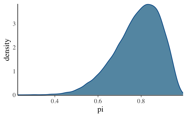
mcmc_hist(bb_sim, pars = "pi") +
  yaxis_text(TRUE) +
  ylab("count")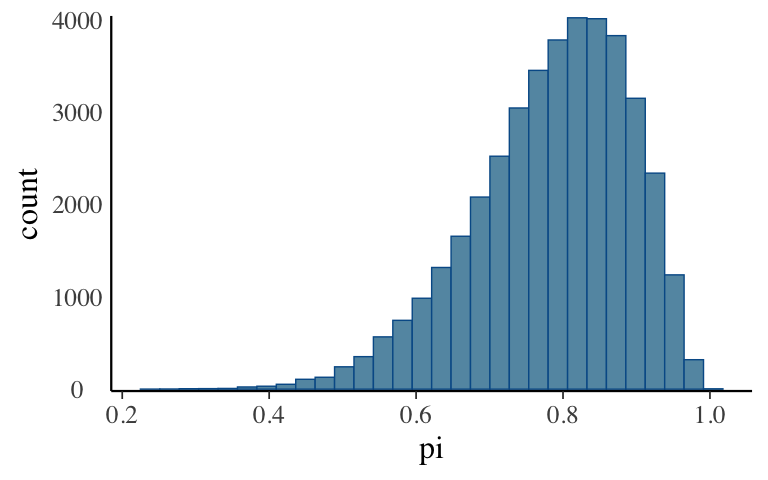
In this illustrative example, we know the posterior is a Beta(11,3) and thus can compare it to our approximation. How did we do?
mcmc_dens(bb_sim, pars = "pi")  +
  stat_function(fun = dbeta, args = list(11, 3), color = "red")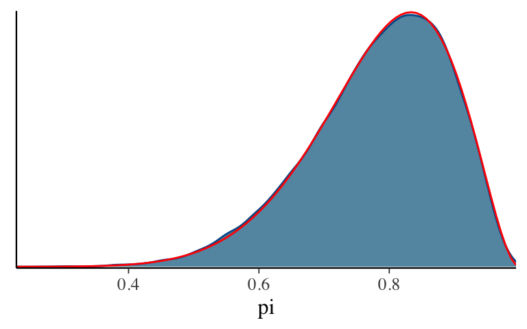
Visual diagnostics: trace plots
Looks pretty random!mcmc_trace(bb_sim, pars = "pi", size = 0.5)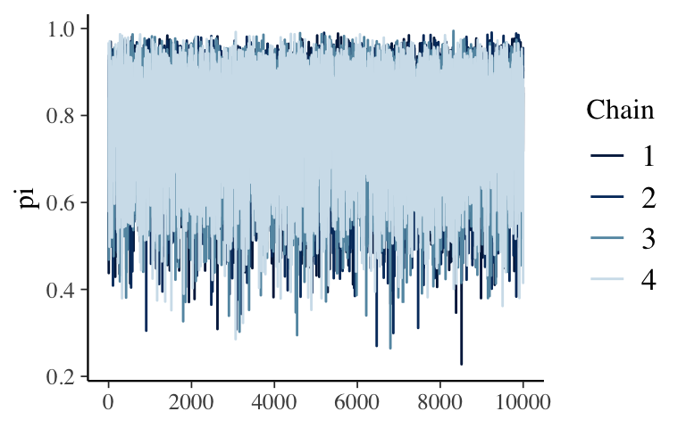
mcmc_trace(bb_sim, pars = "pi", size = 0.5, window = c(0, 100))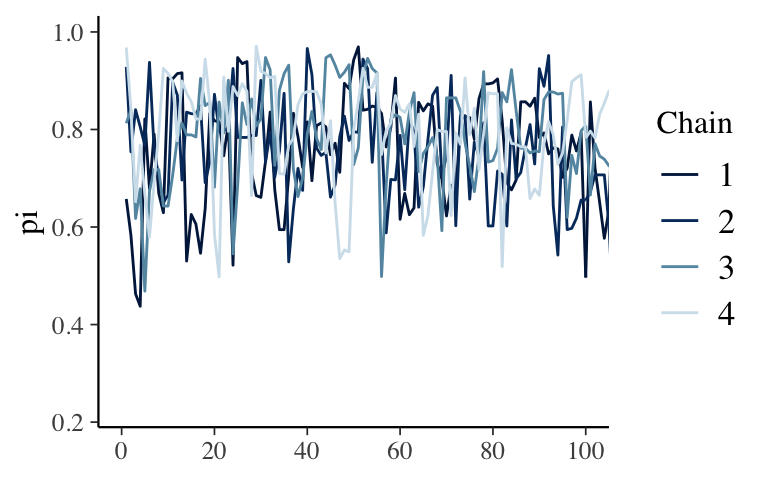
- Visual diagnostics: trace plots continued
- trace 1 –> density B
trace 2 –> density C
trace 3 –> density A
- it should look as random as possible
- if it has some sort of trend / clear correlation among the draws, it will slowly explore the \(\pi\) values, thus will give us a poor approximation if we don’t run the simulation long enough.
if it gets stuck exploring the same values / has flat spots, it will cause erroneous spikes in the posterior approximation - good
- trace 1 –> density B
- Visual diagnostics: Comparing parallel chains
.
# Set the random number seed
set.seed(84735)

# Simulate the posterior
bb_sim_short <- stan(
  model_code = bb_model,
  data = list(alpha = 2, beta = 2, Y = 9, n = 10),
  chains = 4, iter = 100*2)
If the parallel chains produce different posterior approximations, the simulation isn’t stable / trustworthy. Often, this instability can be fixed by running the chain for more iterations. Ideally, we want the different chains to produce similar approximations.
mcmc_dens_overlay(bb_sim, pars = "pi")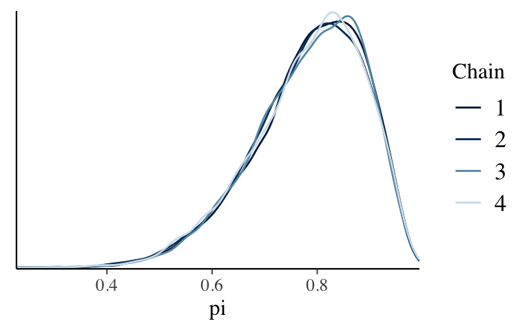
mcmc_dens_overlay(bb_sim_short, pars = "pi")