5 Conjugate families
GOALS
The applicability of the Beta-Binomial model is limited to scenarios in which we’re interested in some proportion \(\pi\) and observe some number of successes \(Y\). Yet there’s more to the world than proportions. We’ll learn some new models today. In the process, we’ll:
Practice model building. When analyzing data, there’s no rule book that will tell you what model is appropriate. Rather, we have to practice some guiding principles and critical thinking.
Learn the foundations of the powerful Normal, Poisson, and logistic regression models that will allow us to study not just the behavior in some lone variable \(Y\), but the relationship between \(Y\) and a set of predictors (\(X_1, X_2, \ldots, X_p\)).
RECOMMENDED READING
Bayes Rules! Chapter 5.
Some handy probability models
| model | support | pmf / pdf |
|---|---|---|
| \(Bin(n,p)\) | \(X \in \{0, 1, \ldots, n\}\) | \(f(x) = \left(\begin{array}{c} n \\ x \end{array} \right) p^x(1-p)^{n-x}\) |
| \(Pois(\lambda)\) | \(X \in \{0, 1, 2, \ldots\}\) | \(f(x) = \frac{\lambda^x e^{-\lambda}}{x!}\) |
| \(Beta(\alpha,\beta)\) | \(X \in [0,1]\) | \(f(x) = \frac{\Gamma(\alpha + \beta)}{\Gamma(\alpha)\Gamma(\beta)} x^{\alpha-1} (1-x)^{\beta-1}\) |
| \(Gamma(s,r)\) | \(X > 0\) | \(f(x) = \frac{r^s}{\Gamma(s)}x^{s-1}e^{-r x}\) |
| \(N(\mu,\sigma^2)\) | \(X \in (-\infty, \infty)\) | \(f(x) = \frac{1}{\sqrt{2\pi\sigma^2}}\exp\left\lbrace - \frac{1}{2}\left(\frac{x-\mu}{\sigma} \right)^2 \right\rbrace\) |
5.1 Warm-up
Review
- Which of the following, per Bayes’ Rule, can we use to calculate the posterior pdf of some parameter \(\theta\) given data \(Y = y\)?
- \(f(\theta | y) = f(\theta)L(\theta | y)\)
- \(f(\theta | y) \propto f(\theta)L(\theta | y)\)
- \(f(\theta | y) = f(y)L(\theta | y) / f(\theta)\)
- \(f(\theta | y) \propto f(y)L(\theta | y)\)
Let \(\pi\) be the proportion of vaccine recipients that are protected against severe illness. A scientist expresses their prior knowledge by \(\pi \sim \text{Beta}(40,20)\). In a study of \(n = 100\) vaccine recipients that got an infection, \(Y = 90\) avoided severe illness. Thus the Beta-Binomial model is:
\[\begin{split} Y | \pi & \sim \text{Bin}(100, \pi) \\ \pi & \sim \text{Beta}(40,20) \\ \end{split} \;\; \Rightarrow \;\; \pi | (Y = 90) \sim \text{Beta}(40 + 90, 20 + 10) = \text{Beta}(130, 30)\]
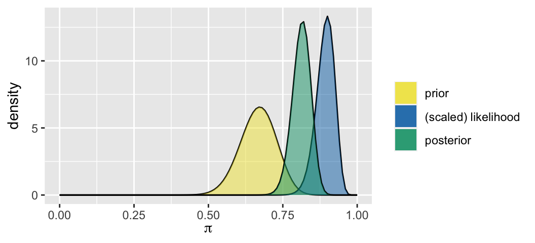
How can we interpret the (scaled) likelihood function of \(\pi\),
\[L(\pi|y=90) = {100 \choose 90}\pi^{90}(1-\pi)^{10} \;\; \text{ for } \pi \in [0,1]\]
- We’re most likely to have seen this 90% protection rate in the study if \(\pi\), the protection rate among the general population, is also around 90%. We’re unlikely to have seen this 90% protection rate if \(\pi\) were as low as 75%.
- Based on this data, \(\pi\) is most likely to be around 90% and is unlikely to be below 75%.
- Prior to observing this data, the scientist understood that \(\pi\) is most likely to be around 90% and is unlikely to be below 75%.
- A different scientist starts with the same prior, but observes the data in two stages. In stage 1, 7 of 10 patients are protected, and in stage 2, 83 of 90 patients are protected. Will this scientist have the same posterior as the previous scientist?
- no
- yes
- no
- The first scientist conducts a second study in which 25 of 30 patients are protected. What’s their posterior model of \(\pi\)?
- Beta(40, 20)
- Beta(40 + 25, 20 + 5) = Beta(65, 25)
- Beta(130 + 25, 30 + 5) = Beta(155, 35)
Write your answers to 1–4 in the blanks below (eg: a/b/c/d, a/b/c, no/yes, g/h/i). Flip the 4th answer upside down.
\[\underline{\hspace{0.75in}} \; \underline{\hspace{0.75in}} \; \underline{\hspace{0.75in}} \; \underline{\hspace{0.75in}}\]
Motivating example
Let \(\pi\) be the proportion of Minnesotans that refer to fizzy drinks as “pop” (not “soda”). To learn about \(\pi\), we poll n adults and record \(Y\), the number that use the word pop.
Why is the Binomial a reasonable conditional model for the dependence of \(Y\) on \(\pi\)?
\[Y|\pi \sim Bin(n, \pi) \;\; \text{ with } \;\; f(y|\pi) = \left(\begin{array}{c} n \\ y \end{array} \right) \pi^y(1-\pi)^{n-y} \;\; \text{ for } y \in \{0,1,\ldots,n\}\]
In light of this conditional model for the data, why is the Beta a reasonable prior model for \(\pi\)?
\[\pi \sim \text{Beta}(\alpha,\beta) \;\; \text{ with } \;\; f(\pi) = \frac{\Gamma(\alpha + \beta)}{\Gamma(\alpha)\Gamma(\beta)} \pi^{\alpha-1} (1-\pi)^{\beta-1} \;\; \text{ for } \pi \in [0,1]\]
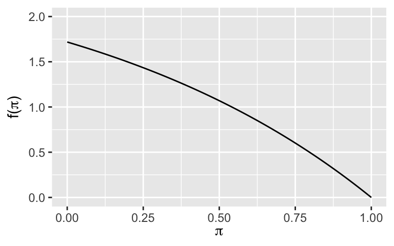
We’ve seen that the Beta prior is conjugate for the Binomial data model, meaning that the posterior will also be a Beta. What if, instead, we utilized a prior model for \(\pi\) with the following pdf:
\[f(\pi) = e - e^\pi \;\; \text{ for } \pi \in [0,1]\]
DEFINITION: conjugate prior
A conjugate prior is one that produces a posterior model in the same “family.” For example, both the prior and posterior in the Beta-Binomial are from the Beta family. Conjugate priors make it easier to build the posterior model and better illustrate the balance that the posterior strikes between the prior and data.
5.2 Exercises
5.2.1 Part 1
- Model 1: data
Let \(\lambda\) be the typical number of mittens that show up in the OLRI lost-and-found on a typical February day. To learn about \(\lambda\), you record data on \(Y\), the number of mittens that show up in the lost-and-found today. What is a reasonable conditional model for the dependence of \(Y\) on \(\lambda\)? State the name of this model and write out its associated likelihood function of \(\lambda\) given data \(Y = y\), \(L(\lambda|y)\). NOTE: Here are some things to think about when identifying a reasonable model.- What values can \(Y\) take? For example, is it a discrete count? Is it continuous?
- Is \(Y\) likely to be symmetric? Skewed?
- What type of model can accommodate these features of \(Y\)?
- Model 1: prior
Next, let’s identify a reasonable prior model for \(\lambda\).- First, what values can \(\lambda\) take? (eg: \(\lambda \in [0,1]\), \(\lambda > 0\), \(\lambda \in \{0,1,2,...\}\), etc)
- In light of the conditional model for data \(Y\), as well as your answer to part a, which of the following do you think would be a reasonable and conjugate prior for \(\lambda\)? Why?
| model | support | pmf / pdf |
|---|---|---|
| \(Bin(n,p)\) | \(\lambda \in \{0, 1, \ldots, n\}\) | \(f(\lambda) = \left(\begin{array}{c} n \\ \lambda \end{array} \right) p^\lambda(1-p)^{n-\lambda}\) |
| \(Pois(l)\) | \(\lambda \in \{0, 1, 2, \ldots\}\) | \(f(\lambda) = \frac{l^\lambda e^{-l}}{\lambda!}\) |
| \(Beta(\alpha,\beta)\) | \(\lambda \in [0,1]\) | \(f(\lambda) = \frac{\Gamma(\alpha + \beta)}{\Gamma(\alpha)\Gamma(\beta)} \lambda^{\alpha-1} (1-\lambda)^{\beta-1}\) |
| \(Gamma(s,r)\) | \(\lambda > 0\) | \(f(\lambda) = \frac{r^s}{\Gamma(s)}\lambda^{s-1}e^{-r \lambda}\) |
| \(N(\mu,\sigma^2)\) | \(\lambda \in (-\infty, \infty)\) | \(f(\lambda) = \frac{1}{\sqrt{2\pi\sigma^2}}\exp\left\lbrace - \frac{1}{2} \left(\frac{\lambda-\mu}{\sigma} \right)^2 \right\rbrace\) |
- Model 1: posterior
Suppose you count up \(Y = y\) mittens. To confirm your hunch from the previous question, specify the posterior model of \(\lambda\) along with any parameters upon which it depends. If your hunch was correct, the prior and posterior will both be from the same model family.
- Model 2: data
Let \(\mu\) be the typical weight of Mac students’ backpacks. To learn about \(\mu\), you randomly sample one student and record \(Y\), the weight of their backpack. Construct an appropriate Bayesian posterior model for \(\mu\).- Which of the following is the most reasonable conditional model for the dependence of \(Y\) on \(\mu\): Bin(\(n,\mu\)), Pois(\(\mu\)), Beta(\(\alpha,\beta\)), or N(\(\mu,\sigma^2\)). Write out the associated likelihood function of \(\mu\), \(L(\mu|y)\).
- There’s a very minor flaw in the model from part a. What is it and why isn’t it a big deal?
- Model 2: prior
Next, let’s identify a reasonable prior model for \(\mu\).- First, according to the conditional model for data \(Y\), what values can \(\mu\) take?
- In light of the conditional model for data \(Y\), as well as your answer to part a, which of the following do you think would be a reasonable and conjugate prior for \(\mu\)? Why?
| model | support | pmf / pdf |
|---|---|---|
| \(Bin(n,p)\) | \(\mu \in \{0, 1, \ldots, n\}\) | \(f(\mu) = \left(\begin{array}{c} n \\ \lambda \end{array} \right) p^\mu(1-p)^{n-\mu}\) |
| \(Pois(\lambda)\) | \(\mu \in \{0, 1, 2, \ldots\}\) | \(f(\mu) = \frac{\lambda^\mu e^{-\lambda}}{\mu!}\) |
| \(Beta(\alpha,\beta)\) | \(\mu \in [0,1]\) | \(f(\mu) = \frac{\Gamma(\alpha + \beta)}{\Gamma(\alpha)\Gamma(\beta)} \mu^{\alpha-1} (1-\mu)^{\beta-1}\) |
| \(Gamma(s,r)\) | \(\mu > 0\) | \(f(\mu) = \frac{r^s}{\Gamma(s)}\mu^{s-1}e^{-r \mu}\) |
| \(N(m,s^2)\) | \(\mu \in (-\infty, \infty)\) | \(f(\mu) = \frac{1}{\sqrt{2\pi s^2}}\exp\left\lbrace - \frac{1}{2}\left(\frac{\mu-m}{s} \right)^2 \right\rbrace\) |
- Model 2: posterior
You will build the posterior for this model in homework 3!
5.2.2 Part 2
In the examples above, we had a single data point \(Y\): the number of lost mittens on 1 day and the weight of 1 backpack. In practice, we typically observe more than one data point: \(\vec{Y} = (Y_1,Y_2,...,Y_n)\). As such, we must consider the joint model which describes the randomness in this entire data collection (not just of one data point). Recall the following result from Probability.
Joint model
Let \(\vec{Y} = (Y_1,Y_2,...,Y_n)\) be an independent random sample where the dependence of each \(Y_i\) on some parameter \(\theta\) is described by pdf
\[f(y_i | \theta)\]
Then the joint dependence of \(\vec{Y}\) on \(\theta\) is described by pdf
\[f(\vec{y} | \theta) = \prod_{i=1}^n f(y_i | \theta) = f(y_1 | \theta)f(y_2 | \theta) \cdots f(y_n | \theta)\]
Challenge: more data
Tune the conjugate prior model of \(\lambda\) to have a mean of 2 and a standard deviation of 1. NOTE: A Gamma(\(s,r\)) model has mean \(s/r\) and variance \(s/r^2\).
Plot this prior using
plot_gamma()inbayesrules.Suppose you observe the following numbers of lost mittens: (0, 1, 2, 0). That is, you observe 0 mittens on day 1, 1 on day 2, 2 on day 3, and 0 on day 4. Build the posterior model of \(\lambda\). (There’s more room on the next page.)
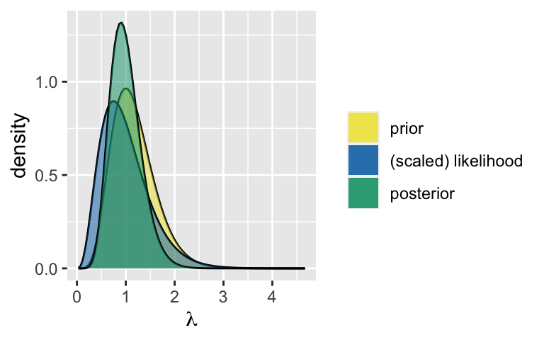
Check out and summarize your Bayesian analysis. Plug your prior parameters into the
shapeandratearguments. Plug the sum of your data points and number of data points intosum_yandn.library(bayesrules) plot_gamma_poisson(shape = ___, rate = ___, sum_y = ___, n = ___)
5.3 Solutions
- Model 1: data
\(Y\) is a positive count with technically no upper bound. Thus it’s reasonable to assume that \[\begin{split} Y | \lambda & \sim Pois(\lambda) \\ L(\lambda|y) & = \frac{\lambda^y e^{-\lambda}}{y!} \;\; \text{ for } \lambda > 0 \\ \end{split}\]
- Model 1: prior
- \(\lambda > 0\)
- \(\lambda \sim Gamma(s,r)\). The Gamma pdf has a similar structure to the Poisson likelihood function.
Model 1: posterior
\[\begin{split} f(\lambda|y) & \propto f(\lambda)L(\lambda|y) \\ & = \frac{r^s}{\Gamma(s)}\lambda^{s-1}e^{-r \lambda} \cdot \frac{\lambda^y e^{-\lambda}}{y!} \\ & \propto \lambda^{s-1}e^{-r \lambda} \lambda^y e^{-\lambda} \\ & = \lambda^{(s + y) -1}e^{-(r + 1) \lambda} \\ \end{split}\]This is a \(Gamma(s + y, r + 1)\) pdf, thus
\[\lambda | y \sim Gamma(s + y, r + 1)\]
- Model 2: data
Normal. \(\mu\) is continuous and isn’t restricted to [0,1].
\[L(\mu|y) = \frac{1}{\sqrt{2\pi \sigma^2}}\exp\left\lbrace -\frac{1}{2}\left(\frac{y - \mu}{\sigma}\right)^2 \right\rbrace\]
Weights can’t be non-negative, whereas the Normal lives on the real line. However, we can put near-0 weight on negative values.
- Model 2: prior
- \(\mu \in (-\infty,\infty)\)
- \(\mu \sim N(m,s^2)\). The prior pdf has similar structure to the Normal likelihood function.
- Model 2: posterior
- Challenge: more data
Gamma(4,2)
.
plot_gamma(4, 2)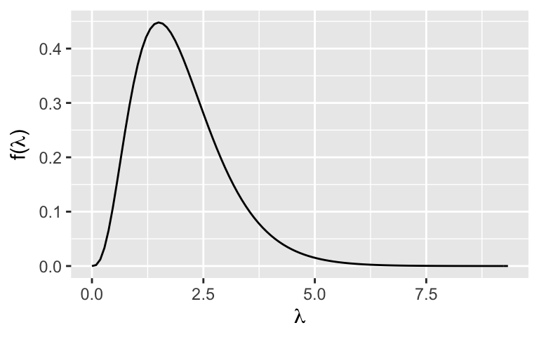
\(\lambda | \vec{Y} \sim \text{Gamma}(7, 6)\). Proof:
\[\begin{split} f(\lambda) & = \frac{2^4}{\Gamma(4)}\lambda^{3}e^{-2\lambda} \\ L(\vec{y} | \lambda) & = \prod_{i=1}^4 f(y_i | \lambda) \\ & = f(y_1 = 0|\lambda)f(y_2 = 1|\lambda)f(y_3 = 2|\lambda)f(y_4 = 0|\lambda) \\ & = \frac{\lambda^0e^{-\lambda}}{0!}\frac{\lambda^1e^{-\lambda}}{1!}\frac{\lambda^{2}e^{-\lambda}}{2!}\frac{\lambda^{0}e^{-\lambda}}{0!} \\ & = \lambda^3e^{-4\lambda} \\ f(\lambda | \vec{y}) & \propto f(\lambda)L(\vec{y} | \lambda) \\ & = \frac{2^4}{\Gamma(4)}\lambda^{3}e^{-2\lambda}\lambda^3e^{-4\lambda} \\ & \propto \lambda^6 e^{-6\lambda} \\ \end{split}\].
plot_gamma_poisson(shape = 7, rate = 6, sum_y = 3, n = 4)