8 Posterior prediction
GOALS
Once we’ve built or simulated a Bayesian posterior, not only might we want construct estimates and assess hypotheses, we might want to use our model to make predictions for future data.
RECOMMENDED READING
Bayes Rules! Chapter 8.
8.1 Warm-up
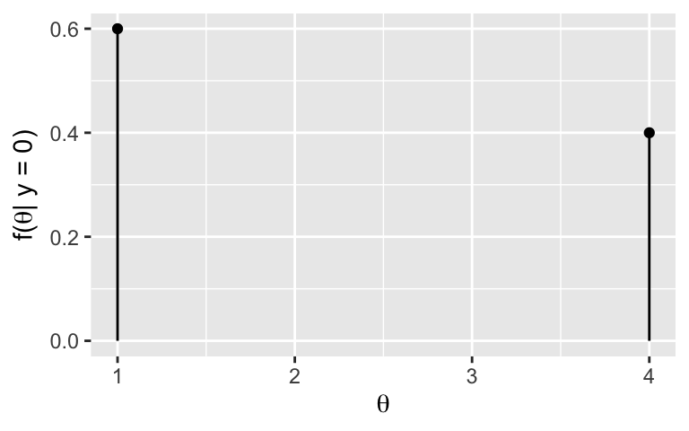
We’re playing a game in which our friend flips a fair coin \(\theta \in \{1,4\}\) times and then records \(Y\), the number of Heads. The friend doesn’t tell us \(\theta\), but does tell us \(Y\). And based on a past analysis in which we observed \(Y = 0\), suppose we have the following posterior model of \(\theta\):
| \(\theta\) | 1 | 4 |
|---|---|---|
| \(f(\theta|y=0)\) | 0.6 | 0.4 |
WARM-UP 1
Let \(Y'\) be the number of Heads that your friend gets the next time they flip the coin \(\theta\) times. What’s your best guess for \(Y'\): 0, 1, 2, 3, or 4? Why?
WARM-UP 2
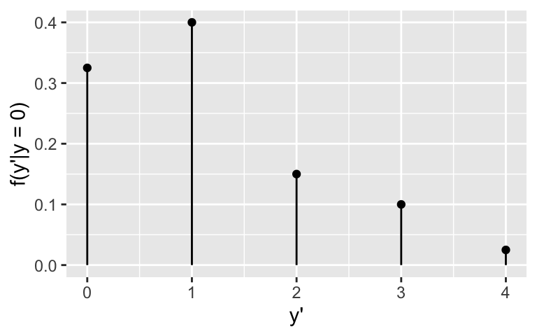
Of course, there’s more than one possible outcome for \(Y'\):
Thus instead of providing a single best guess, it’s important to build a complete posterior predictive model for \(Y'\). Like any probability model, this defines the possible outcomes of \(Y'\) and the relative plausibility of these outcomes. Prove that this posterior predictive model has the following pmf:
| \(y'\) | 0 | 1 | 2 | 3 | 4 |
|---|---|---|---|---|---|
| \(f(y'| y = 0)\) | 0.325 | 0.4 | 0.15 | 0.1 | 0.025 |
Posterior prediction models
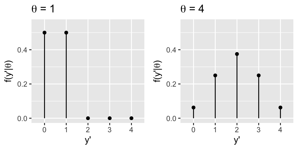
Let \(f(\theta | y)\) be the posterior pdf/pmf of \(\theta\) given we observed data \(Y = y\). To predict a new data outcome \(Y'\) we have to consider two sources of variability:
sampling variability in the data
\(Y'\) can take on more than one value. This randomness in \(Y'\) is defined by its conditional pdf/pmf, \(f(y' | \theta)\).posterior variability in \(\theta\)
Some values of \(\theta\) are more plausible than others. This randomness in \(\theta\) is defined by the posterior pdf/pmf \(f(\theta | y)\).
Then to build the posterior predictive model of \(Y'\), we can weight the chance of observing \(Y' = y'\) for any given \(\theta\) by the posterior plausibility of \(\theta\):
\[\begin{array}{rlr} f(y' | y) & = \int f(y'|\theta)f(\theta|y)d\theta & \;\; \text{ (when $\theta$ is continuous)} \\ f(y' | y) & = \sum_\theta f(y'|\theta)f(\theta|y) & \;\; \text{ (when $\theta$ is discrete)} \\ \end{array}\]
8.2 Exercises
Let \(\pi \in [0,1]\) be the proportion of U.S. adults that don’t believe in climate change. Starting with a Beta(1,2) prior for \(\pi\), and observing a survey in which \(Y = 150\) of \(n = 1000\) surveyed adults didn’t believe in climate change, we built a Beta(151, 852) posterior model for \(\pi\):
\[\begin{split} Y|\pi & \sim Bin(1000,\pi) \\ \pi & \sim Beta(1, 2) \\ \end{split} \;\; \Rightarrow \;\; \pi | (Y = 150) \sim Beta(151, 852)\]
library(bayesrules)
plot_beta_binomial(alpha = 1, beta = 2, y = 150, n = 1000) +
    xlim(0.1, 0.2)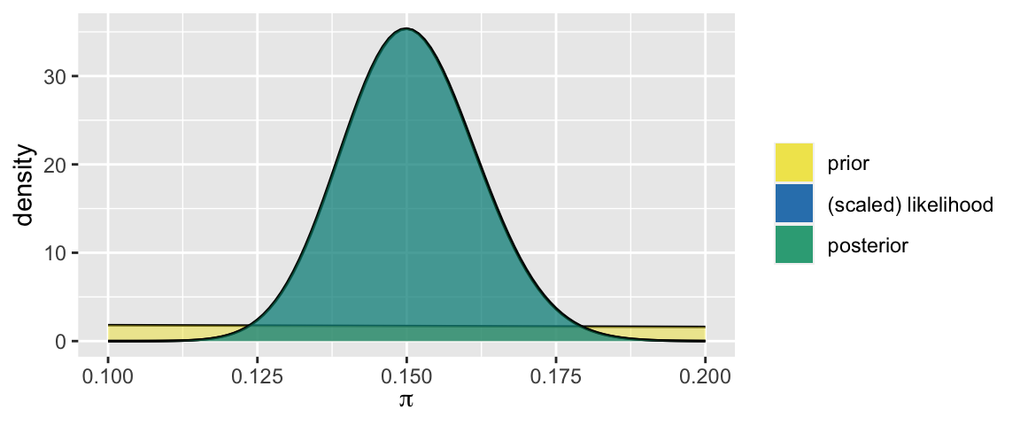
- Best guess
We plan to survey 20 more people and want to predict \(Y'\), the number that don’t believe in climate change. Recall that the posterior mode of \(\pi\) was around 0.15. With this, what’s your best guess of \(Y'\)?
Simulation
In the previous activity, you used MCMC simulation to approximate the posterior model of \(\pi\):# Load some necessary packages library(rstan) library(rstanarm) library(bayesrules) library(bayesplot) library(broom.mixed) # Import the MCMC simulation results climate_sim <- readRDS(url("https://www.macalester.edu/~ajohns24/data/stat454/climate_sim.rds")) # Store the array of 4 chains in 1 data frame climate_chains <- as.data.frame( climate_sim, pars = "lp__", include = FALSE) # Check out the results dim(climate_chains) head(climate_chains)We can use this MCMC simulation to approximate the entire posterior model of \(Y'\). Specifically, utilizing the 20,000 posterior plausible \(\pi\) values in
climate_chains, simulate a sample of predictions \(Y'\) and print out the first 6 rows. NOTE:- The 20,000 chain values capture one source of variability: posterior variability in \(\pi\). To capture the other source, sampling variability in the data, first think about the model for \(Y' | \pi\).
- Since this is a random process, be sure to
set.seed()for reproducibility.
- Follow-up
- Construct a graphical summary of the (approximated) posterior predictive model of \(Y'\). NOTE: \(Y'\) should be integer values from 0 to 20. If it’s not, go back to the previous exercise and try another technique.
- What’s the most likely value of \(Y'\)?
- Approximate an 80% prediction interval for \(Y'\).
- Approximate the probability that more than 5 of the 20 people won’t believe in climate change.
Optional: Math
Consider the general Beta-Binomial setting:\[\begin{split} Y|\pi & \sim Bin(n,\pi) \\ \pi & \sim Beta(\alpha, \beta) \\ \end{split} \;\; \Rightarrow \;\; \pi | (Y = y) \sim Beta(\alpha + y, \beta + n - y)\]
Let \(Y'\) denote the number of successes in the next \(m\) trials (where \(m\) might be different from \(n\)). Not only can we simulate the posterior predictive model of \(Y'\), we can specify it mathematically. Prove that the posterior predictive pmf of \(Y'\) is
\[\begin{split} f(y'|y) & = \int f(y'|\pi) f(\pi|y) d\pi \\ & = \left(\begin{array}{c} m \\ y' \end{array} \right) \frac{\Gamma(\alpha + \beta + n)}{\Gamma(\alpha + y)\Gamma(\beta+n-y)} \frac{\Gamma(\alpha + y + y')\Gamma(\beta+n-y+m-y')}{\Gamma(\alpha + \beta + n + m)} \\ \end{split}\]
8.3 Solutions
- Best guess
\(0.15*20 \approx 3\)
Simulation
# Load some necessary packages
library(rstan)
library(rstanarm)
library(bayesrules)
library(bayesplot)
library(broom.mixed)

# Import the MCMC simulation results
climate_sim <- readRDS(url("https://www.macalester.edu/~ajohns24/data/stat454/climate_sim.rds"))

# Store the array of 4 chains in 1 data frame
climate_chains <- as.data.frame(
  climate_sim,
  pars = "lp__", include = FALSE)

# Check out the results
head(climate_chains)
##          pi
## 1 0.1551602
## 2 0.1466082
## 3 0.1471497
## 4 0.1508684
## 5 0.1641593
## 6 0.1651653
# Set the random number seed set.seed(84735) # Simulate 1 Binomial prediction Y' from each pi climate_chains <- climate_chains %>% mutate(y_new = rbinom(20000, size = 20, prob = pi)) # Check it out head(climate_chains) ## pi y_new ## 1 0.1551602 4 ## 2 0.1466082 4 ## 3 0.1471497 3 ## 4 0.1508684 5 ## 5 0.1641593 5 ## 6 0.1651653 2
Follow-up
# a
ggplot(climate_chains, aes(x = y_new)) +
  geom_bar()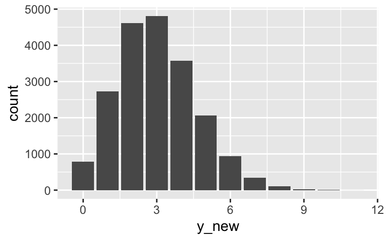
# b
# 3

# c
climate_chains %>%
  summarize(quantile(y_new, 0.1), quantile(y_new, 0.9))
##   quantile(y_new, 0.1) quantile(y_new, 0.9)
## 1                    1                    5

# d
climate_chains %>%
  summarize(mean(y_new > 5))
##   mean(y_new > 5)
## 1         0.07055