1 Bayesian Statistics?!?

1.1 A Quiz

For each question below, circle the statement with which you most strongly agree. Go with your gut instead of what you might’ve learned in past courses. There are no right or wrong answers here!

1. When flipping a fair coin, ‘the probability of flipping Heads is 0.5.’ How do you interpret this probability?
   1. If I flip this coin over and over and over and over, roughly 50% of the flips will be Heads.
      
   2. If I flip this coin, Heads / Tails are equally plausible.
      
   3. Both of the above make sense.

2. An election is coming up and a pollster claims that ‘candidate A has a 0.9 probability of winning.’ How do you interpret this probability?
   1. If we observe the election over and over, candidate A will win roughly 90% of the time.
   2. Candidate A is much more likely to win than to lose.
   3. The pollster’s calculation is wrong. Candidate A will either win or lose, thus their probability of winning can only be 0 or 1.

3. I survey 10 Mac students and perform 2 experiments:
   • I ask each student if they plan to vote for Trump in 2024. 10 out of 10 say “yes.”
     
   • I give each student a sample of coffee and a sample of chai tea. 10 out of 10 correctly identify which sample is which.
   In light of these experiments, what do you conclude?
   1. You’re more confident that Mac students can distinguish between coffee & chai than that Mac students plan to vote for Trump.
   2. The evidence in favor of Mac students’ intention to vote Trump is just as strong as the evidence in favor of Mac students’ ability to identify between coffee and chai.

4. In a study of 20 people, you observed the following relationship between stress and sleep:
   

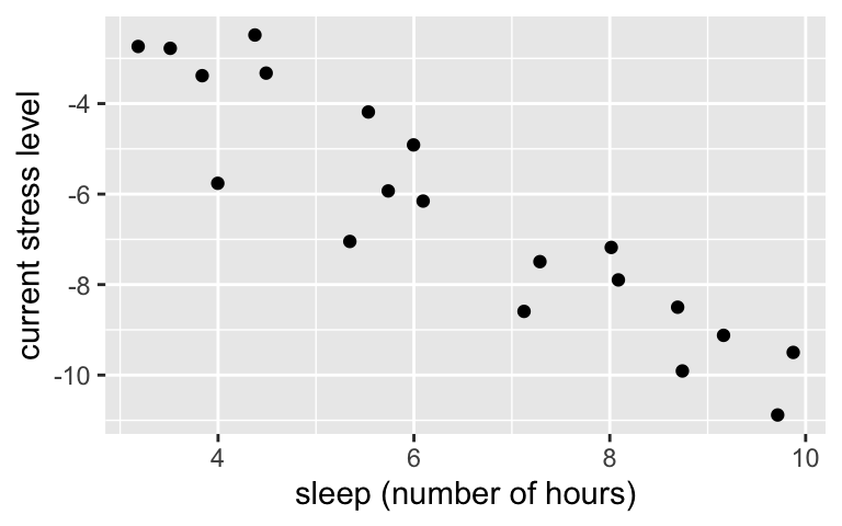
   What’s the next question you ask yourself?

   1. If in fact there’s no association between stress and sleep, what’s the chance that I would’ve seen such a strong relationship in this sample of 20 people?
      
   2. Based on the observed data on these 20 people, what’s the chance that there’s an association between stress and sleep?

AFTER YOU FINISH YOUR QUIZ

Calculate & interpret your score:

2. 1. 1 point
   2. 3 points
   3. 2 points
3. 1. 1 point
   2. 3 points
   3. 1 point
4. 1. 3 points
   2. 1 point
5. 1. 1 point
   2. 3 points

Interpret Your Score:

• 4-5 = Fairly frequentist
• 6-9 = Who needs to choose sides?
• 10-12 = Big Bayesian

Then get into 4 groups:

• Make sure that at least 1 member of your group took MATH 354 last semester.
  
• Meet each other and discuss what you’re most excited about this semester.
  
• Calculate your average quiz score.
  
• Discuss your assigned quiz problem.
  
• Summarize this all in front of the class!

1.2 Bayesian vs frequentist statistics

Both Bayesians and frequentists seek to learn from data, using data to fit models, make predictions, and evaluate hypotheses. Moreover, when working from the same data, Bayesians and frequentists will typically arrive at a similar set of broad conclusions. Yet there are key differences in the logic behind, approach to, and interpretation of Bayesian and frequentist analyses.

Concept	Frequentist interpretation	Bayesian interpretation
probability	the long-run relative frequency of a repeatable event (hence “frequentist”")	a measure of the relative plausibility of an event
role of data	data alone should drive our outgoing information	data should be weighed against our incoming information
questions asked	If the hypothesis isn’t correct, what are the chances I’d have observed these data?	In light of these data, what are the chances the hypothesis is correct?

1.3 Exercises

Goal: Review some foundational Probability concepts

No matter when you took Probability, be patient with yourself. Whether you haven’t taken Probability in a while or you took it under the module structure, it will likely take some time to jump back in and feel comfortable. This is natural. You’ll get there! We’ll review the 3 types of probability models.

Model	Purpose	Probability mass function (pmf)
Marginal	describe the behavior of a single variable (ignoring all other variables)	\(f(x)\) describes possible values of \(X\) and the relative plausibility of each
Joint	describe the simultaneous behavior of 2+ variables	\(f(x,y)\) describes possible pairs of (\(X\),\(Y\)) values and the relative plausibility of each
Conditional	describe how the behavior of one variable depends upon another	\(f(x|y)\) describes possible values of \(X\) when \(Y = y\) and the relative plausibility of each

The story

You’re playing a thrilling game of Dungeons & Dragons. During your turn, the DM tells you to roll a 4-sided die two times:⁴

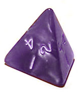
Let \(X\) be the minimum value of the two rolls & \(Y\) be the maximum. Thus \(X\) and \(Y\) are discrete random variables – they can vary from roll to roll and can take on a discrete set of outcomes. These equally likely possible outcomes are summarized below.

1. Marginal models of discrete \(X\) and \(Y\)
   Consider the marginal outcomes of \(X\) and \(Y\) alone:

   \[f(x) = P(X = x) \;\; \text{ and } \;\; f(y) = P(Y = y)\]

   1. Write out the pmfs for \(X\) and \(Y\) in table form. Use decimals, not fractions.

      \(x\)	1	2	3	4	Total
      \(f(x)\)	\(\hspace{.5in}\)	\(\hspace{.5in}\)	\(\hspace{.5in}\)	\(\hspace{.5in}\)	\(\hspace{.5in}\)

      
      

      \(y\)	1	2	3	4	Total
      \(f(y)\)	\(\hspace{.5in}\)	\(\hspace{.5in}\)	\(\hspace{.5in}\)	\(\hspace{.5in}\)	\(\hspace{.5in}\)

   2. Convince yourself that we can also write \(f(x)\) and \(f(y)\) in equation form: \[\begin{split} f(x) & = 0.5625 - 0.125x \;\; \text{ for } x \in \{1,2,3,4\} \\ f(y) & = 0.125y - 0.0625 \;\; \text{ for } y \in \{1,2,3,4\} \\ \end{split}\]

   
   

   3. Calculate \(\sum_{\text{all $x$}} f(x)\) and \(\sum_{\text{all $y$}} f(y)\). NOTE: \(\sum\) = sum.

2. Joint model of \(X\) and \(Y\)
   The marginal pmfs above merely describe the separate outcomes of the min and max rolls. Yet in our game, it’s the combination of these that matters. For example, if the minimum roll is even and the maximum roll is odd, perhaps we get to cast a magic spell! Thus we want to model the joint behavior of \((X,Y)\) by the joint pmf for \(X\) and \(Y\): \[f(x,y) = P(\{X = x\} \; \cap \; \{Y=y\})\] Recall: \(\cap\) = “and” or “intersection.”

   1. Summarize \(f(x,y)\) in the table below. Again, use decimals not fractions.

   		y
   	\(f(x,y)\)	1	2	3	4	Total
   \(x\)	1	\(\hspace{.25in}\)	\(\hspace{.25in}\)	\(\hspace{.25in}\)	\(\hspace{.25in}\)	\(\hspace{.25in}\)
   	2
   	3
   	4
   	Total

   
   

   2. Summarize \(f(x,y)\) in formula form:
      \[f(x,y) = \begin{cases} ??? & x < y \\ ??? & x = y \\ ??? & x > y \\ \end{cases}\]

   3. Calculate the total of the pmf across all possible combinations of \(x\) and \(y\): \[\sum_{\text{all $x$}}\sum_{\text{all $y$}} f(x,y)\]

   4. Where have you seen the far right column before? That is, what happens when we sum \(f(x,y)\) across all possible \(y\)?

      \[\sum_{\text{all $y$}} f(x,y) = ???\]

      This property is guaranteed by the Law of Total Probability.

LAW OF TOTAL PROBABILITY: connecting the joint & marginal models

In general, \(f(x)\) describes the of observing \(X = x\) across all values of \(Y\). Thus, \(f(x)\) can be obtained by summing the joint pmf across all possible values of \(Y\): \[f(x) = \sum_y f(x,y)\] Similarly, \(f(y)\) describes the overall chance of observing \(Y = y\) across all values of \(X\): \[f(y) = \sum_x f(x,y)\]

3. Conditional probabilities
   The DM is a trickster. They roll but don’t show you their 2 dice. Instead, they present you with some puzzles…

   1. What’s the probability that the min value is 3? \[P(\{X = 3\}) = \; ???\]

   
   

   2. My maximum value is 2. What’s the conditional probability that the minimum is 3? \[P(\{X = 3\} \; | \; \{Y = 2\}) = ???\]

      		y
      	\(f(x,y)\)	1	2	3	4	Total
      \(x\)	1	0.0625	0.125	0.125	0.125	0.4375
      	2	0	0.0625	0.125	0.125	0.3125
      	3	0	0	0.0625	0.125	0.1875
      	4	0	0	0	0.0625	0.0625
      	Total	0.0625	0.1875	0.3125	0.4375	1

   
   

   3. My maximum value is 3. What’s the conditional probability that the minimum is 2? \[P(\{X = 2\} \; | \; \{Y = 3\}) = ???\]

      		y
      	\(f(x,y)\)	1	2	3	4	Total
      \(x\)	1	0.0625	0.125	0.125	0.125	0.4375
      	2	0	0.0625	0.125	0.125	0.3125
      	3	0	0	0.0625	0.125	0.1875
      	4	0	0	0	0.0625	0.0625
      	Total	0.0625	0.1875	0.3125	0.4375	1

Conditional models

The conditional probability of observing \(X=x\) when \(Y=y\) is calculated by scaling the joint probability of observing this \((x,y)\) combination by the overall chance of observing \(Y = y\) in the first place: \[P(\{X = x\} | \{Y = y\}) = \frac{P(\{(X = x\} \cap \{Y = y\})}{P(Y = y)}\] In pmf notation, the conditional model of \(X\) given \(Y = y\) is the ratio of their joint model and the marginal model of \(Y\): \[f(x|y) = \frac{f(x,y)}{f(y)}\]

NOTE:

In the conditional model of \(X\) given \(Y = y\), \(X\) is the random variable and \(y\) is a fixed constant. Thus like all valid pmfs, \(f(x|y)\) must sum to 1 across all possible values of random variable \(X\): \[\sum_x f(x|y) = 1\]

4. Conditional model of \(X\) when \(Y = 3\)
   Again, assume the DM tells us that their maximum roll was \(Y = 3\).

   1. Define the conditional model of the minimum roll, \(X\), in light of the information that \(Y=3\):

      \(x\)	1	2	3	4	Total
      \(f(x|(y=3))\)

   
   

   2. Calculate \(\sum_{x = 1}^4 f(x|(y=3))\).

5. Conditional model of \(X\) when \(Y = y\)

   Let’s generalize the above work to other possible information about \(Y\). To do so, you’ll need the marginal pmf from exercise 1 and the joint pmf from exercise 2: \[\begin{split} f(y) & = 0.125y - 0.0625 \;\; \text{ for } y \in \{1,2,3,4\} \\ f(x,y) & = \begin{cases} 0.1250 & x < y \\ 0.0625 & x = y \\ 0 & x > y \\ \end{cases} \end{split}\]

   1. Combine \(f(y)\) with \(f(x,y)\) to construct the conditional pmf of \(X\) given \(Y = y\): \[f(x|y) =\frac{f(x,y)}{f(y)} = \hspace{4.5in}\]

   2. Does \(\sum_{x = 1}^4 f(x|y)\) necessarily equal 1?

   3. Does \(\sum_{y=1}^4 f(x|y)\) necessarily equal 1?

6. Independence
   1. Did the information that \(Y = 3\) change our understanding of \(X\)? Explain.
      
   2. Are \(X\) and \(Y\) independent variables?

Independent variables

Conceptually, random variables \(X\) and \(Y\) are independent if information about \(Y\) doesn’t change our understanding of \(X\). Formally, \(X\) and \(Y\) are independent if and only if \[f(x|y) = f(x)\]
Equivalently, \(X\) and \(Y\) are independent if and only if \[f(x,y) = f(x)f(y)\]

1.4 Solutions

1. .

   1. .

      \(x\)	1	2	3	4	Total
      \(f(x)\)	0.4375	0.3125	0.1875	0.0625

      \(y\)	1	2	3	4	Total
      \(f(y)\)	0.0625	0.1875	0.3125	0.4375

   2. For example, \(f(x = 1) = 0.5625 - 0.125*1 = 0.4375\)

   3. \(\sum_{\text{all $x$}} f(x) = 1\) and \(\sum_{\text{all $y$}} f(y) = 1\).

2. .
   1. See the Law of Total Probability box.
   2. See exercise 3.
      
   3. \(\sum_{\text{all $x$}}\sum_{\text{all $y$}} f(x,y) = 1\)
      
   4. The far right column is just the pmf of \(X\) and the far bottom row is the pmf of \(Y\).

3. .

   1. \(f(x=3) = 0.1875\)

   2. \(f((x=3)|(y=2)) = f((x=3),(y=2)) / f(y=2) = 0\). Or, simply note that it’s impossible for the min to be bigger than the max!

   3. \(f((x=2)|(y=3)) = f((x=2),(y=3)) / f(y=3) = 0.125/0.3125 = 0.4\)

4. .

   1. .

      \(x\)	1	2	3	4	Total
      \(f(x|(y=3))\)	0.4	0.4	0.2	0	1

   2. \(\sum_{x = 1}^4 f(x|(y=3)) = 1\)

5. .

   1. \[f(x|y) =\frac{f(x,y)}{f(y)} = \begin{cases} \frac{0.1250}{0.125y - 0.0625} & x < y \\ \frac{0.0625}{0.125y - 0.0625} & x = y \\ 0 & x > y \\ \end{cases}\]

   2. Yes. It’s a model of \(X\) when \(Y=y\), thus the pmf of this model sums to 1.

   3. No. This is a model of \(X\), not \(Y\).

6. .
   1. Yes. It removed \(X=4\) from the realm of possibilities and changed the probabilities of the remaining possible outcomes.
   2. No. Knowing that \(Y=3\) changed what we understood about \(X\)

---

4. photo: https://commons.wikimedia.org/wiki/File:4-sided_dice_250.jpg↩︎