Unit overview
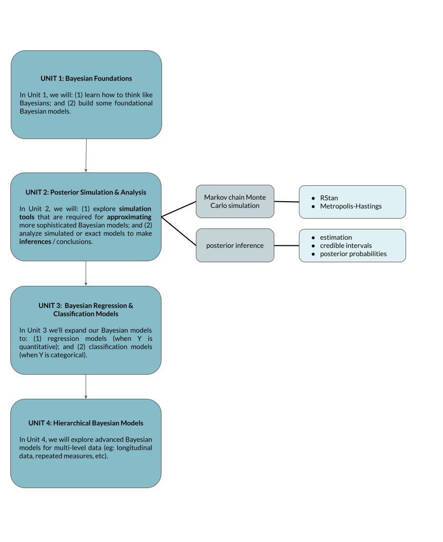
Motivation
We’ll soon move onto studying advanced Bayesian models for which it’s prohibitively difficult, if not impossible, to mathematically specify the posterior:
\[f(\theta|y) = \frac{f(y|\theta)f(\theta)}{f(y)} = ???\]
Approach
Simulate a sample with features similar to that of the posterior.
Use this sample to approximate the posterior & its features.
Tools
Suppose we wish to approximate a posterior model of \(\theta\) with pdf \(f(\theta | y)\).
Monte Carlo A Monte Carlo sample \[\left\lbrace \theta^{(1)}, \theta^{(2)}, \ldots, \theta^{(N)}\right\rbrace\] is a random sample of size \(N\) from posterior \(f(\theta|y)\). That is:
the \(\theta^{(i)}\) are independent of one another
each \(\theta^{(i)}\) is drawn directly from \(f(\theta|y)\).
Limitations: Monte Carlo simulation can be computationally inefficient and break down when the “universe” or sample space of \(Y\) is continuous or large. Similarly, it breaks down when we have and are simulating more than one model parameter \(\theta\).
grid approximation
Grid approximation is intuitive and easy to implement but is limited to simpler Bayesian models.Markov chain Monte Carlo (MCMC)!!
Markov chain Monte Carlo methods can scale up for more sophisticated Bayesian models, but at a cost. A Markov chain \[\left\lbrace \theta^{(1)}, \theta^{(2)}, \ldots, \theta^{(N)}\right\rbrace\] is NOT a random sample of size \(N\) from posterior \(f(\theta|y)\):each chain value \(\theta^{(i+1)}\) is drawn from a model that depends upon the current state \(\theta^{(i)}\): \[g\left(\theta^{(i+1)} \; \vert \; \theta^{(i)},y\right)\]
and chain values are not drawn from the posterior
\[g\left(\theta^{(i+1)} \; \vert \; \theta^{(i)},y\right) \ne f\left(\theta^{(i+1)} \; \vert \; y \right)\]
BUT when done efficiently, a Markov chain sample will mimic a random sample which converges to and provides a good approximation of the posterior.
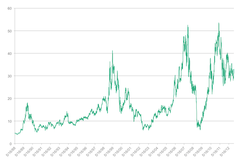
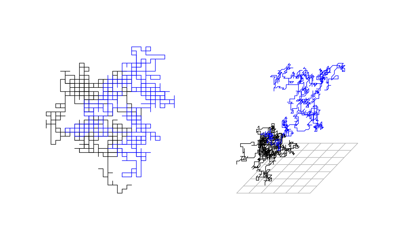
OTHER APPLICATIONS
Their application to Bayesian modeling is our motivation to study MCMC. However, they enjoy countless other applications. For example, \(\left\lbrace \theta^{(1)}, \theta^{(2)}, \ldots\right\rbrace\) might be: stock prices5, steps in a “dizzy walk” (a classic), or the path of a molecule:
Or a chain of text (eg: text generation, tweet generation (from Prof Bryan Martin), text decryption), or musical notes (example).
An MCMC plan for this course:
What does MCMC output look like and how do we know if it’s “good?”
How can we utilize MCMC output for posterior analysis, including estimation, testing, and prediction?
How do MCMC algorithms work?6
Markov chains are my area of expertise! Though I’d love to spend the entire semester talking about them, in the interest of exploring more sophisticated models, we’ll focus on the concepts over the details. If you want to think about the details, this might be a good Capstone topic.↩︎