13 Poisson & Negative Binomial regression
INTERNATIONAL ROUNDTABLE
This year’s International Roundtable is on Student protests: Unsettling power relationships and cultivating radical hope. Data activism is just one example of how this topic connects to the MSCS classroom. You can earn 10 homework points for attending one of the events and writing up the following:
- A 1–2 sentence summary of what you took away from the session. What surprised you the most? What made you think the most?
- 1 question you asked or would like to ask the presenter(s).
- A 2–3 sentence discussion of an example, real or hypothetical, that connects the session’s topic to data activism.
GOALS
Not everything is Normal (luckily). Let’s expand our regression models to other types of quantitative response variables \(Y\).
Continue to practice our Bayesian workflow.

RECOMMENDED READING
Bayes Rules! Chapter 12.
13.1 Warm-up
WARM-UP 1: Just \(Y\)
Suppose we’re interested in the number of anti-discrimination laws that a state has, \(Y\). What’s an appropriate model for the variability in \(Y_i\) from state to state? NOTE: In practice, the number of laws tends to be right-skewed.
- \(Y_i | \pi \stackrel{ind}{\sim} \text{Bin}(1, \pi)\) with \(E(Y_i | \pi) = \pi\)
- \(Y_i | \lambda \stackrel{ind}{\sim} \text{Pois}(\lambda)\) with \(E(Y_i | \lambda) = \lambda\)
- \(Y_i | \mu, \sigma \stackrel{ind}{\sim} N(\mu, \sigma^2)\) with \(E(Y_i | \mu, \sigma) = \mu\)
WARM-UP 2: Adding a predictor (step 1)
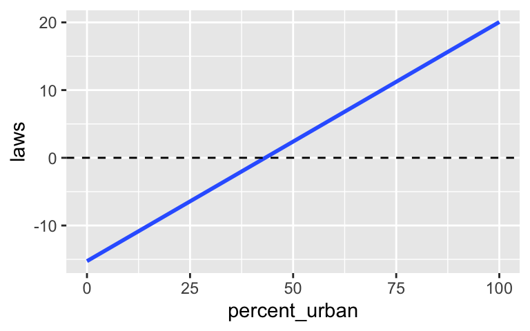
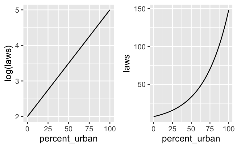
Suppose we wished to predict how many anti-discrimination laws a state has, \(Y\), by the percent of its residents that live in urban areas, \(X\). Modify your model from the first warm-up example to incorporate the age predictor \(X\). In doing so, explain why it’s better to assume that
\[\log(E(Y|X)) = \beta_0 + \beta_1 X\]
than that
\[E(Y|X) = \beta_0 + \beta_1 X\]
The plot below might help.
WARM-UP 3: Finalizing the Bayesian model
Upon what parameters does your model depend?
What are appropriate prior models for these parameters (e.g. Beta, Gamma, Normal)?
The Bayesian Poisson regression model
To model response variable \(Y\) by predictor \(X\), suppose we collect \(n\) data points. Let \((Y_i, X_i)\) denote the observed data on each case \(i \in \{1, 2, \ldots, n\}\). Then the Bayesian Poisson regression model is as follows:
\[\begin{array}{rll} Y_i | \beta_0, \beta_1, \sigma & \stackrel{ind}{\sim} \text{Pois}(\lambda_i) & \text{where } \log(\lambda_i) = \beta_0 + \beta_1 X_i \\ && \text{equivalently, } \lambda_i = e^{\beta_0 + \beta_1 X_i}\\ \beta_{0c} & \sim N(m_0, s_0^2) & \\ \beta_1 & \sim N(m_1, s_1^2) & \\ \end{array}\]
NOTES:
The priors on \((\beta_0, \beta_1)\) are independent of one another.
For interpretability, we state our prior understanding of the model intercept \(\beta_0\) through the centered intercept \(\beta_{0c}\).
When \(X = 0\), \(\beta_0\) is the expected logged \(Y\) value and \(e^{\beta_0}\) is the expected \(Y\) value.
For each 1-unit increase in \(X\), \(\beta_1\) is the expected change in the logged \(Y\) value and \(e^{\beta_1}\) is the expected multiplicative change in \(Y\). That is
\[\beta_1 = \log(\lambda_{x+1}) - \log(\lambda_x) \;\; \text{ and } \;\; e^{\beta_1} = \frac{\lambda_{x+1}}{\lambda_x}\]
WARM-UP 4: Interpreting Poisson coefficients
As a simple example, consider the following model of a state’s number of anti-discrimination laws by its urban percentage:
\[\log(\lambda) = 2 + 0.05X \;\; \text{ and } \lambda = e^{2 + 0.05X}\]
How can we interpret \(\beta_0 = 2\) and \(e^{\beta_0} \approx 7.39\)? For states that have 0% of its residents in urban areas…
How can we interpret \(\beta_1 = 0.05\) and \(e^{\beta_1} \approx 1.05\)? For each extra percentage point in urban population…
13.2 Exercises
NOTE: The extra practice exercises are included to help complete the Bayesian modeling workflow and to provide more practice with concepts from previous activities. You are encouraged to skip these for now and return to them once you’ve completed the other exercises.
13.2.1 Part 1
The equality_index data in the bayesrules package includes the observed number of anti-discrimination laws in each state, \(Y\). Below you’ll model \(Y\) by a state’s percent_urban and its historical presidential voting patterns. The historical variable has 3 levels:
dem= the state typically votes for the Democratic candidategop= the state typically votes for the Republican (GOP) candidateswing= the state often swings back and forth between Democratic and Republican candidates
# Load packages
library(tidyverse)
library(tidybayes)
library(rstan)
library(rstanarm)
library(bayesplot)
library(bayesrules)
library(broom.mixed)

# Load data
data("equality_index")

# Remove California, an extreme outlier with 155 laws
equality <- equality %>%
    filter(state != "california")
Not Normal
Before diving into Poisson regression, let’s convince ourselves it’s necessary. Simulate the posterior Normal regression model:# Simulate the posterior Normal regression model normal_model <- stan_glm( laws ~ percent_urban + historical, data = equality, family = gaussian, chains = 4, iter = 5000*2, seed = 84735, refresh = 0)Next, construct a posterior predictive check of the model to determine if it’s wrong (it is). NOTE: The darks curve in this plot is misleading. The observed
lawsare all non-negative, but the curve is filled in to match the range of the x-axis.# Construct a posterior predictive check #___ + # geom_vline(xintercept = 0) + # xlab("laws")
- Simulate Poisson priors
That was bad. Let’s move on the Poisson regression model.Simulate weakly informative priors for this regression model by changing ONE line in the code below. NOTE: The function automatically logs the \(Y\) variable for Poisson regression, so don’t change this in our formula.
EXTRA PRACTICE: Summarize the prior tunings and fill in the model structure below.
\[\begin{split} Y_i | \beta_0, \beta_1, \beta_2, \beta_3 & \stackrel{ind}{\sim} \text{Pois}(\lambda_i) \;\; \text{ with } \log(\lambda_i) = \beta_0 + \beta_1 X_1 + \beta_2 X_2 + \beta_3 X_3 \\ \beta_{0c} & \sim N(???, ???^2) & \\ \beta_1 & \sim N(???, ???^2) & \\ \beta_2 & \sim N(???, ???^2) & \\ \beta_3 & \sim N(???, ???^2) & \\ \end{split}\]
# Simulate the prior Poisson regression model
prior_poisson <- stan_glm(
  laws ~ percent_urban + historical, data = equality,
  family = gaussian,
  prior_PD = TRUE,
  chains = 4, iter = 5000*2, seed = 84735, refresh = 0)

# EXTRA PRACTICE: Check the prior tunings
Prior simulation
Use the plot below to describe our prior understanding of the relationship between anti-discrimination laws, urban percentage, and historical voting patterns. NOTE: Theylim()is included since the range of the models is so wide.equality %>% add_fitted_draws(prior_poisson, n = 200) %>% ggplot(aes(x = percent_urban, y = laws, color = historical)) + geom_line(aes(y = .value, group = paste(historical, .draw))) + ylim(0, 100)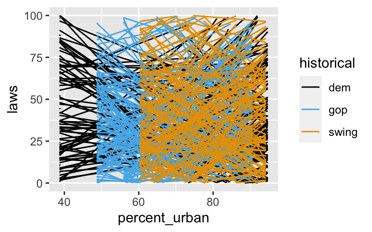
- Check out the data
With the prior in place, consider the data. Construct and summarize a plot oflawsvspercent_urbanandhistorical.
- Posterior simulation & MCMC diagnostics
- Simulate the posterior model and perform a quick posterior predictive check to ensure we’re now on the right track.
- EXTRA PRACTICE: Construct 2 visual summaries that allow you to diagnose whether the MCMC simulation has stabilized (i.e. whether we should trust the simulation results).
- Simulate the posterior model and perform a quick posterior predictive check to ensure we’re now on the right track.
- Posterior analysis
Check out 200 posterior plausible model curves:
# equality %>% # add_fitted_draws(YOUR POSTERIOR MODEL, n = 200) %>% # ggplot(aes(x = percent_urban, y = laws, color = historical)) + # geom_line(aes(y = .value, group = paste(historical, .draw)), alpha = 0.1) + # geom_point()Obtain and interpret posterior median estimates for the
swingandpercent_urbancoefficients. Do so on the unlogged scale.
Posterior prediction
Minnesota has a 73.3% urban percentage and has historically voted for Democrats in presidential elections. (History tidbit: The Democrat winning streak is longer in Minnesota than any other state.)mn <- equality %>% filter(state == "minnesota") mn ## # A tibble: 1 x 6 ## state region gop_2016 laws historical percent_urban ## <fct> <fct> <dbl> <dbl> <fct> <dbl> ## 1 minnesota midwest 44.9 4 dem 73.3- Predict the number of anti-discrimination laws in Minnesota using the shortcut
posterior_predict()function. Plot and describe the posterior predictive model. NOTE:- You can plug
mndirectly intoposterior_predict(). - In plotting the shortcut, use
mcmc_hist() with abinwidth = 1`.
- You can plug
- In reality, Minnesota has 4 anti-discrimination laws. How does this compare to our predictive model?
- EXTRA PRACTICE: Repeat part a from scratch, i.e. without the shortcut function.
- Predict the number of anti-discrimination laws in Minnesota using the shortcut
- Model evaluation: is the model fair?
Though the data collection process was honest, there are reasons to be cautious when interpreting and reporting this model. For example:- What would you say to somebody that used this model to claim that
demstates tend to have better anti-discrimination laws? - What would you say to somebody that used this model to claim that a person in a
gopstate supports discrimination?
- What would you say to somebody that used this model to claim that
- EXTRA PRACTICE: Model evaluation: How accurate are the posterior predictions?
Use visual and cross-validated numerical summaries to assess the quality of our posterior model predictions.
13.2.2 Part 2
Consider a new model. Our goal will be to explore how \(Y\), the typical number of books that a person reads each year, is related to their age (\(X_1\)) and their response to the question “would you rather be wise but unhappy or happy but unwise?”:
\[X_2 = \begin{cases} 1 & = \text{ wise but unhappy} \\ 0 & = \text{ happy but unwise} \\ \end{cases}\]
To this end, we’ll use the survey responses from the Pulse of the Nation dataset:
# Load data
data(pulse_of_the_nation)
# Remove an outlier
pulse <- pulse_of_the_nation %>%
filter(books < 100)First, simulate the posterior Normal regression model which assumes
\[Y_i | \beta_0, \beta_1, \beta_2, \sigma \sim N(\mu_i, \sigma^2) \;\; \text{ with } \mu_i = \beta_0 + \beta_1 X_{i1} + \beta_2 X_{i2}\]
# Simulate the Normal regression model
books_normal <- stan_glm(
books ~ age + wise_unwise, data = pulse,
family = gaussian,
chains = 4, iter = 5000*2, seed = 84735, refresh = 0)Second, simulate the posterior Poisson regression model which assumes
\[Y_i | \beta_0, \beta_1, \beta_2 \sim \text{Pois}(\lambda_i) \;\; \text{ with } \log(\lambda_i) = \beta_0 + \beta_1 X_{i1} + \beta_2 X_{i2}\]
# Simulate the Poisson regression model
books_poisson <- stan_glm(
books ~ age + wise_unwise, data = pulse,
family = poisson,
chains = 4, iter = 5000*2, seed = 84735, refresh = 0)
- Bad models
- Before checking any simulation results, which do you think is more appropriate, the Normal or Poisson regression model? Why?
- Construct a posterior predictive check for both models. Are they good? If not, summarize the discrepancies between the posterior simulations and the observed data.
- Before checking any simulation results, which do you think is more appropriate, the Normal or Poisson regression model? Why?
Overdispersed data
It turns out that the Poisson probability model is pretty rigid. If \(Y \sim \text{Pois}(\lambda)\), then its mean and variance are equal:\[E(Y) = Var(Y) = \lambda\]
For example, if \(Y \sim Pois(25)\), then its mean and variance are both equal to 25. Contrast this with the Normal, whose bell-shaped densities can have any combination of mean and variance. For example, a Normal model with a mean of 25 can have a variance of 25 (\(Y \sim N(25, 5^2)\)) or any other positive variance (eg: a much bigger variance of 100, \(Y \sim N(25, 10^2)\)).
Calculate the variance and mean of the
booksoutcomes to show that thebooksoutcomes do not come close to meeting this rigid Poisson assumption. Specifically, the variance in book readership from person to person far exceeds the average book readership. (The same is true for book readership among people in any given age bracet with similar answers to the wisdom vs happiness question.)NOTE: When the observed variance in \(Y\) exceeds the variance expected by the assumed probability model (here Poisson), we say the data are overdispersed.
Alternatively, use the
pp_check()to argue that the observed data are overdispersed in comparison to the simulated outcomes from the Poisson regression model.
The Negative Binomial probability model
The Negative Binomial probability model is a less rigid alternative to the Poisson. (It’s also the last new probability model we’ll use this semester!) Let \(Y\) be some count in \(\{0, 1, 2, \ldots\}\). Further, for mean parameter \(\mu\) and reciprocal dispersion parameter \(r\), suppose\[Y | \mu, r \sim NegBin(\mu, r)\]
with pdf
\[f(y|\mu,r) = {y + r - 1 \choose r}\left(\frac{r}{\mu + r}\right)^r\left(\frac{\mu}{\mu + r}\right)^y \;\; \text{ for } y \in \{0,1,2,\ldots\}\]
Then \(Y\) has unequal mean and variance:
\[E(Y|\mu,r) = \mu \;\; \text{ and } \;\; Var(Y|\mu,r) = \mu + \frac{\mu^2}{r}\]
Use these properties of the mean and variance to support the following claims about the comparisons between the Negative Binomial and Poisson models.
- For large \(r\), the Negative Binomial and Poisson models have similar properties.
- For small \(r\) close to 0, the Negative Binomial model is overdispersed in comparison to a Poisson model with the same mean.
Further support these claims by simulating and comparing samples from the Pois(5), NegBinom(5,10000), and NegBinom(5,1) models.
# Simulate the samples set.seed(84735) sim_data <- data.frame( u = rpois(1000, 5), v = rnbinom(1000, mu = 5, size = 10000), x = rnbinom(1000, mu = 5, size = 1)) # Plot the samples ggplot(sim_data, aes(x = u)) + geom_bar() + lims(x = c(-1, 32), y = c(0, 200)) + labs(title = "Pois(5)") ggplot(sim_data, aes(x = v)) + geom_bar() + lims(x = c(-1, 32), y = c(0, 200)) + labs(title = "NegBinom(5, 10000)") ggplot(sim_data, aes(x = x)) + geom_bar() + lims(x = c(-1, 32), y = c(0, 200)) + labs(title = "NegBinom(5, 1)")
Negative Binomial regression
To use this more flexible model, we can simply swap out the Poisson for the Negative Binomial model for our regression analysis:\[Y_i | \beta_0, \beta_1, \beta_2 \sim \text{NegBinom}(\mu_i, r) \;\; \text{ with } \log(\mu_i) = \beta_0 + \beta_1 X_{i1} + \beta_2 X_{i2}\]
- Simulate the posterior Negative Binomial regression model,
neg_binomial_2instan_glm()syntax. - Perform a posterior predictive check to ensure that we’re now on the right track.
- What do the data tell us? Plot the relationship between
books,age, andwise_unwise. - Explore a
tidy()posterior summary which includes 95% credible intervals. What does it indicate about book readership?
- Simulate the posterior Negative Binomial regression model,
- NEXT UP
Just a friendly reminder that to really absorb the material, you should do the following after you complete this or any other activity:- review the exercises
- check your work with the solutions
- organize & take additional notes
- note what you still have questions on, and ask these questions in class, OH, or on Slack. maybe even read the recommended reading!
13.3 Solutions
Not Normal
# Construct a posterior predictive check pp_check(normal_model) + geom_vline(xintercept = 0) + xlab("laws")
Simulate Poisson priors
\[\begin{split} Y_i | \beta_0, \beta_1, \beta_2, \beta_3 & \stackrel{ind}{\sim} \text{Pois}(\lambda_i) \;\; \text{ with } \log(\lambda_i) = \beta_0 + \beta_1 X_1 + \beta_2 X_2 + \beta_3 X_3 \\ \beta_{0c} & \sim N(0, 2.5^2) & \\ \beta_1 & \sim N(0, 0.17^2) & \\ \beta_2 & \sim N(0, 4.97^2) & \\ \beta_3 & \sim N(0, 5.60^2) & \\ \end{split}\]# Simulate the prior Poisson regression model prior_poisson <- stan_glm( laws ~ percent_urban + historical, data = equality, family = poisson, prior_PD = TRUE, chains = 4, iter = 5000*2, seed = 84735, refresh = 0) # Check the prior tunings prior_summary(prior_poisson) ## Priors for model 'prior_poisson' ## ------ ## Intercept (after predictors centered) ## ~ normal(location = 0, scale = 2.5) ## ## Coefficients ## Specified prior: ## ~ normal(location = [0,0,0], scale = [2.5,2.5,2.5]) ## Adjusted prior: ## ~ normal(location = [0,0,0], scale = [0.17,4.97,5.60]) ## ------ ## See help('prior_summary.stanreg') for more details
Prior simulation
equality %>%
  add_fitted_draws(prior_poisson, n = 200) %>%
  ggplot(aes(x = percent_urban, y = laws, color = historical)) +
    geom_line(aes(y = .value, group = paste(historical, .draw))) +
    ylim(0, 100)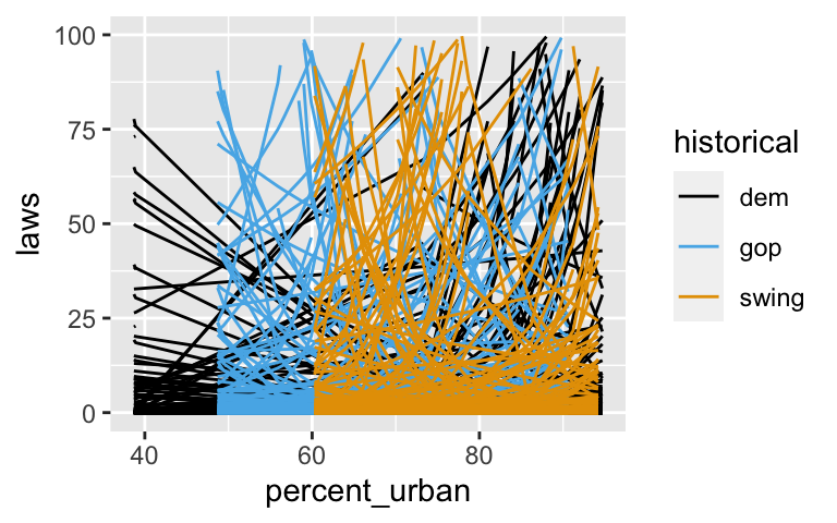
Check out the data
It seems that states with higher urban populations, anddemstates, tend to have more anti-discrimination laws.ggplot(equality, aes(x = percent_urban, y = laws, color = historical)) + geom_point()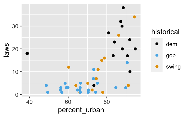
Posterior simulation & MCMC diagnostics
# Simulate the posterior posterior_poisson <- update(prior_poisson, prior_PD = FALSE) # Perform MCMC diagnostics (looks stable!) mcmc_trace(posterior_poisson)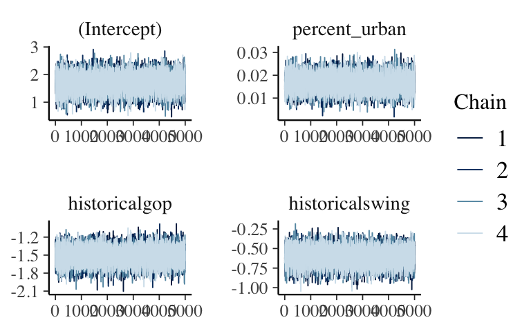
mcmc_dens_overlay(posterior_poisson)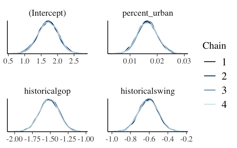
# Posterior predictive check (looks much better!) pp_check(posterior_poisson)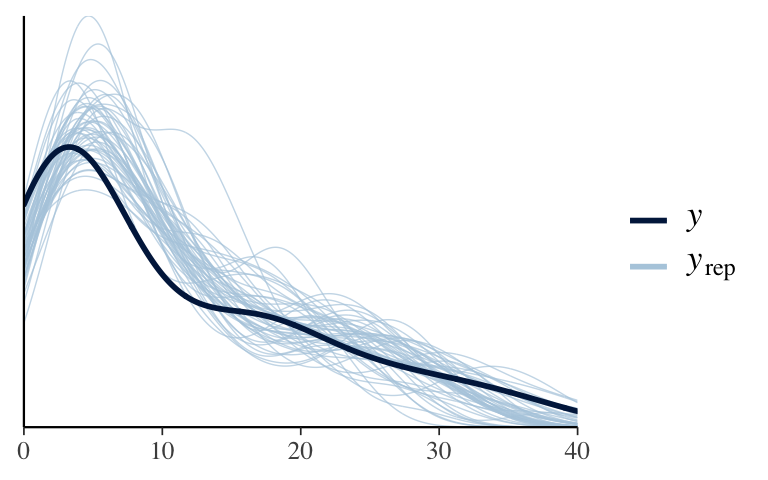
Posterior analysis
When controlling for urban percentage,swingstates tends to have 54% as many anti-discrimination laws as ademstate. When controlling for historical voting trends, for each percentage point increase in urban population, the number of anti-discrimination laws tend to increase by 1.65%.tidy(posterior_poisson, conf.int = TRUE, conf.level = 0.95) ## # A tibble: 4 x 5 ## term estimate std.error conf.low conf.high ## <chr> <dbl> <dbl> <dbl> <dbl> ## 1 (Intercept) 1.71 0.311 1.08 2.29 ## 2 percent_urban 0.0164 0.00361 0.00947 0.0237 ## 3 historicalgop -1.52 0.136 -1.79 -1.26 ## 4 historicalswing -0.608 0.106 -0.817 -0.403 # Transform coefficients of the log scale exp(-0.608) ## [1] 0.5444387 exp(0.0164) ## [1] 1.016535
Posterior prediction
The posterior predictive model expected a much larger number of anti-discrimination laws.# Posterior prediction from scratch set.seed(84735) as.data.frame(posterior_poisson) %>% mutate(y_mn = rpois(20000, lambda = exp(`(Intercept)` + percent_urban*73.3))) %>% ggplot(aes(x = y_mn)) + geom_bar()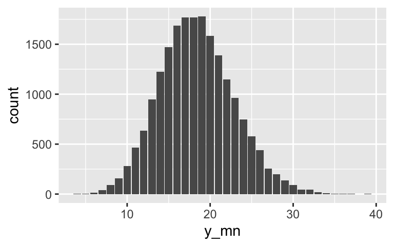
# Posterior prediction using the shortcut set.seed(84735) posterior_predict(posterior_poisson, newdata = mn) %>% mcmc_hist(binwidth = 1)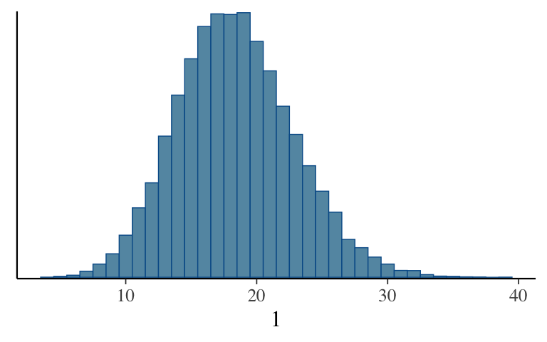
- Model evaluation: is the model fair?
- A greater number of laws doesn’t necessarily mean that the overall quality of laws is better.
- Our analysis tells us about state-level trends, thus cannot be used to infer the actions / beliefs of any individual.
Model evaluation: How accurate are the posterior predictions?
The predictions aren’t that great. The posterior means tend to be off by 3.8 laws and roughly only 72.5% of observed law outcomes will be within the 95% prediction intervals.# First obtain posterior predictive models # for each data point in weather: set.seed(84735) predictions <- posterior_predict(posterior_poisson, newdata = equality) # Plot the posterior predictive intervals ppc_intervals_grouped( equality$laws, yrep = predictions, x = equality$percent_urban, group = equality$historical, prob = 0.5, prob_outer = 0.95, facet_args = list(scales = "fixed")) + labs(x = "percent_urban", y = "laws")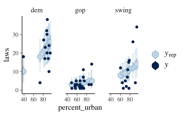
# Calculate CV metrics set.seed(84735) prediction_summary_cv(model = posterior_poisson, data = equality, k = 10)$cv ## mae mae_scaled within_50 within_95 ## 1 3.782268 1.265585 0.3 0.725
- Bad models
Poisson.
booksare counts.
Both are bad.
pp_check(books_normal)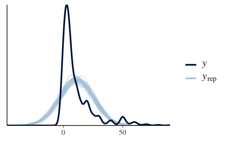
pp_check(books_poisson)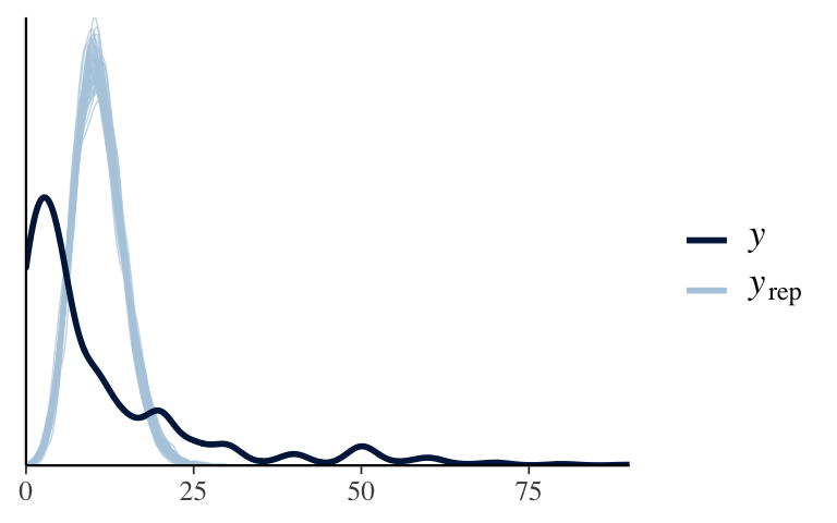
Overdispersed data
In thepp_check(), the observed data have a smaller mean and a much bigger variance. Further, the observed book counts have a variance that’s 10 times as large as the mean (nowhere near equal).equality %>% summarize(mean(laws), var(laws)) ## # A tibble: 1 x 2 ## `mean(laws)` `var(laws)` ## <dbl> <dbl> ## 1 10.6 106.
- The Negative Binomial probability model
- For large \(r\), \(E(Y) \approx Var(Y)\), just like with the Poisson model.
- For small \(r\), \(Var(Y) > E(Y)\).
When \(r = 10000\) (big), the NegBinom(5,10000) is very similar to the Pois(5). When \(r = 1\), the NegBinom(5,1) has the same mean as the Pois(5) but is relatively overdispersed (has a much bigger variance).
# Simulate the samples set.seed(84735) sim_data <- data.frame( u = rpois(1000, 5), v = rnbinom(1000, mu = 5, size = 10000), x = rnbinom(1000, mu = 5, size = 1)) # Plot the samples ggplot(sim_data, aes(x = u)) + geom_bar() + lims(x = c(-1, 32), y = c(0, 200)) + labs(title = "Pois(5)")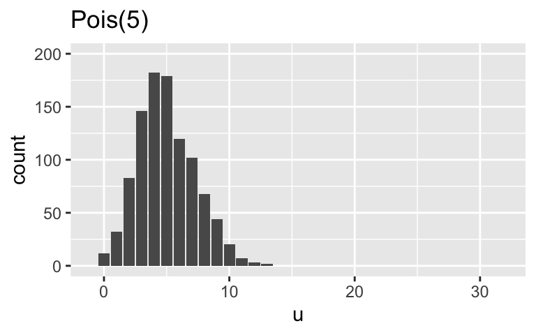
ggplot(sim_data, aes(x = v)) + geom_bar() + lims(x = c(-1, 32), y = c(0, 200)) + labs(title = "NegBinom(5, 10000)")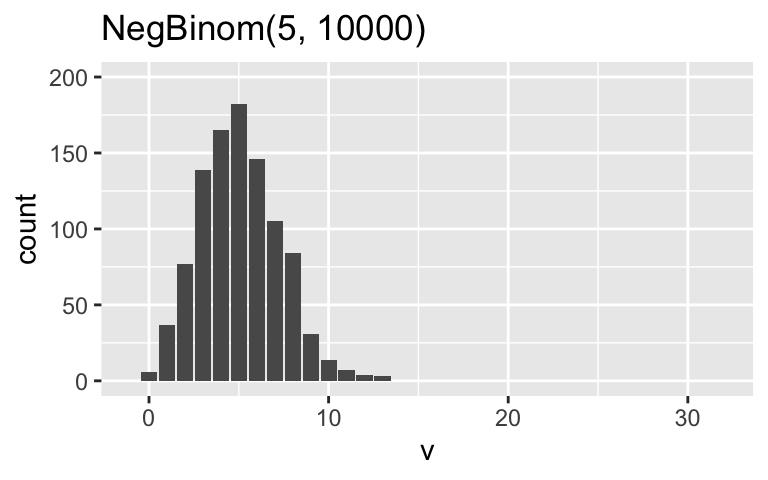
ggplot(sim_data, aes(x = x)) + geom_bar() + lims(x = c(-1, 32), y = c(0, 200)) + labs(title = "NegBinom(5, 1)")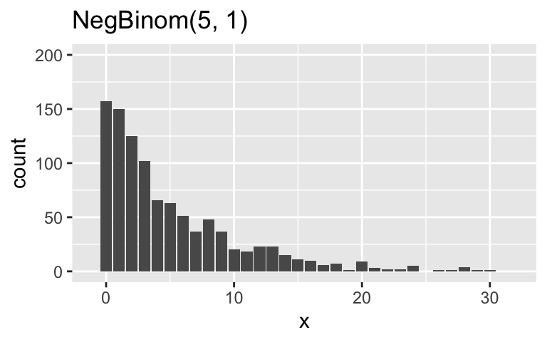
Negative Binomial regression
# a. Simulate the posterior Negative Binomial regression model
books_negbin <- stan_glm(
  books ~ age + wise_unwise, data = pulse,
  family = neg_binomial_2,
  chains = 4, iter = 5000*2, seed = 84735, refresh = 0)

# b. Posterior predictive check (looks much better!)
pp_check(books_negbin)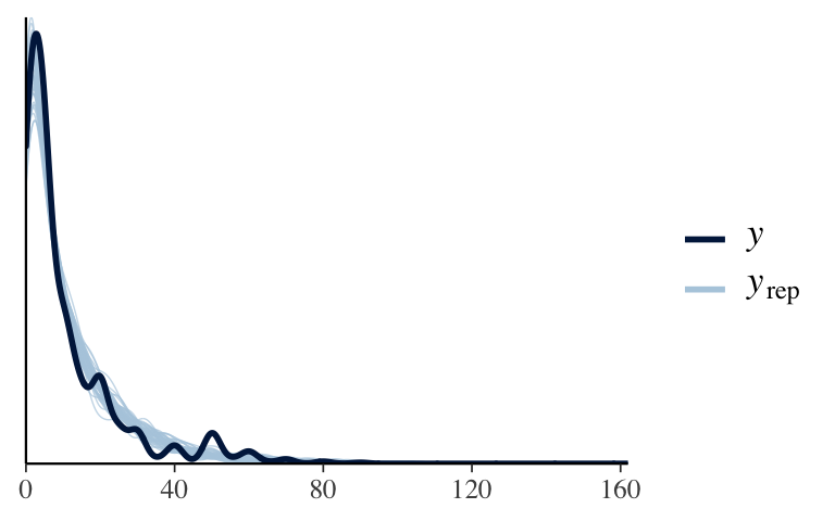
# c. Plot the observed relationship
ggplot(pulse, aes(y = books, x = age, color = wise_unwise)) +
  geom_point()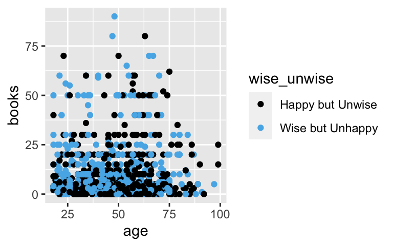
# d. Posterior summary
tidy(books_negbin, conf.int = TRUE, conf.level = 0.95)
## # A tibble: 3 x 5
##   term                        estimate std.error conf.low conf.high
##   <chr>                          <dbl>     <dbl>    <dbl>     <dbl>
## 1 (Intercept)                 2.23       0.131    1.98      2.50
## 2 age                         0.000365   0.00239 -0.00433   0.00501
## 3 wise_unwiseWise but Unhappy 0.266      0.0798   0.111     0.422
exp(0.111)
## [1] 1.117395
exp(0.422)
## [1] 1.525009
When controlling for responses to the wisdom vs happiness question, it doesn’t seem that readership is significantly associated with age (the CI covers 0). When controlling for age, people that prefer wisdom to happiness tend to read somewhere from 12% to 53% more books.