1 Welcome!

Settling in

NOTE: Any spots that open in this course have already been promised to some students from the waitlist. If you’re on the waitlist and I promised you a spot, please stay! If you’re on the waitlist but I have not promised you a spot, I do not anticipate being able to get you into the course :( (thus it is not a good use of your time to stay).
Sit in groups of 3-4. Your group should include:
- nobody that you already know
- at least 1 person who has used RStudio before
Meet the people at your table. Share your names and pronouns. Discuss a high point of your summer break.
You don’t need to take notes today. Everything is in the online manual, which you’ll want to have open in class:
- https://ajohns24.github.io/155_Fall_2025/ (also linked in Moodle)
- left side bar > Simple Linear Regression > 1 Welcome!

Welcome

Statistical Modeling?!

Statistical Modeling is the art and science of turning data into information about relationships of interest. For example, the following are just a few Mac faculty / offices that use statistical models to study relationships:

Michelle Tong (BIOL): Making “Good” Choices: Social Isolation in Mice Exacerbates the Effects of Chronic Stress on Decision Making
Ariel James (PSYCH): Language Experience Predicts Eye Movements During Online Auditory Comprehension
Sarah West (ECON): Redevelopment along arterial streets: The effects of light rail on land use change
Athletics uses data to help understand various relationships (eg: sleep & outcomes, strength over time, etc)

This class is designed for you.

STAT 155 is a modern, non-traditional introduction to statistics. We’ll explore sophisticated tools that typically aren’t covered until a second course in statistics.
- This means:
  - Non-majors taking this as a terminal course will take away highly applicable and marketable knowledge & skills.
  - Majors will gain a solid foundation from which to study more more advanced models & theory.
- This does NOT mean that we’re skipping a course! STAT 155 teaches introductory statistics content, but through a different lens than a traditional course (regression). Relatedly…
Thriving in STAT 155 is NOT correlated with the following: your major, whether you think you’re a “math person,” whether you have any previous idea what “statistical modeling” is, etc. It IS correlated with effort (time, practice, studying, completing assignments without relying on AI) and engagement (attendance, attention, collaboration).
STAT 155 emphasizes statistical applications and intuition over theory (and memorizing formulas). To do that, we’ll utilize statistical software (R/RStudio). It’s assumed that you are totally new to RStudio! More on this later…
I love teaching this course and hope you keep an open mind about it (and all courses you’re taking)!

Introductions & Data Principles

GOAL

Get to know one another a bit better while exploring some basic principles of statistical modeling / working with data.

EXAMPLE 1: Tidy data

You filled out a quick survey before class. The result is a tidy data set! Meaning:

each row = a case or unit of observation (here, a student)
each column = a measure on some variable of interest, which is either…
- quantitative (numbers with units), e.g. age
- categorical (discrete possibilities or categories), e.g. major
each entry contains a single data value; no analysis, summaries, footnotes, comments, etc

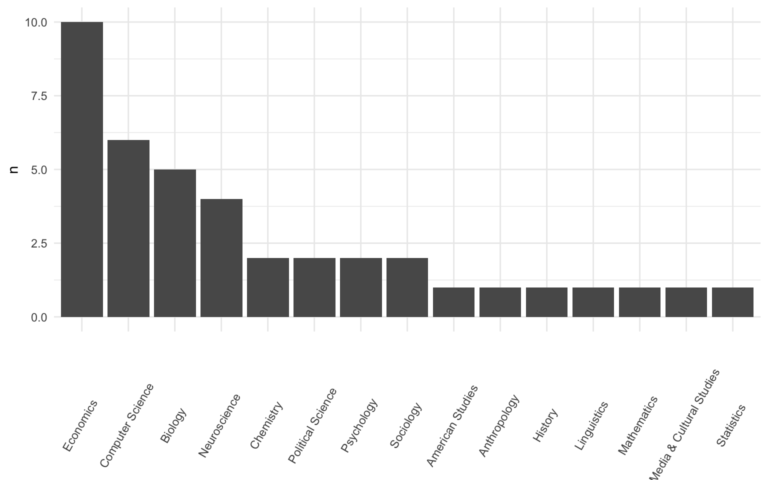
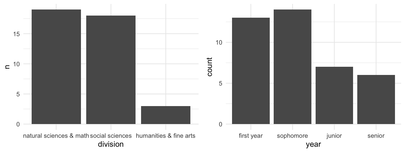
EXAMPLE 2: Academic interests

Below are 3 plots of students’ majors, major divisions, and years in school.

Summarize what you learned about the students in this class.
Suppose a researcher wants to use these data to learn about the academic interests among the broader Mac student body. Is this a good idea? Why or why not?

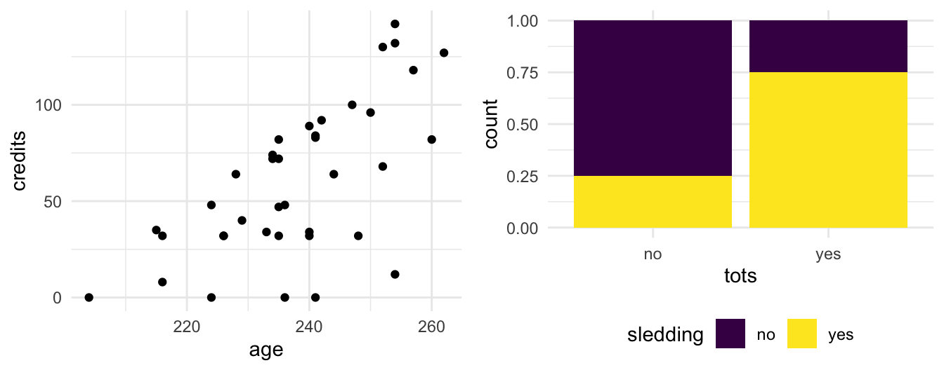
EXAMPLE 3: Relationships

Left plot: Check out the relationship between the number of credits somebody has earned (y-axis) vs their age in months (x-axis). Describe what you observe.
Right plot: Check out the relationship between students’ prior experience with trying tater tot hotdish and trying sledding. Describe what you observe.
After observing this plot, your friend comments that if we give somebody free hotdish, they’ll be more likely to try sledding. Do you agree?

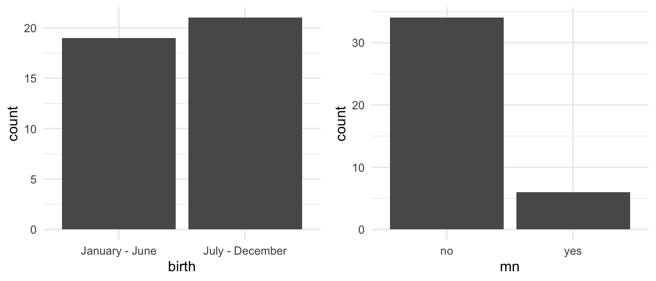
EXAMPLE 4: Conclusions

Pause to make sure you’re still in sync as a group!!

Check out the breakdown of students’ birth months (left plot).
- Are more students born in the 1st or 2nd half of the year?
- Assuming that this class is representative of the broader student body, does this provide substantial evidence of a broader birth trend at Mac?
Check out the breakdown of whether students lived in MN before attending Mac (right).
- Did fewer than half of students in this class live in MN before?
- Assuming that this class is representative of the broader student body, does this provide substantial evidence that fewer than half of Mac students lived in MN before?

PAUSE

Once you’re finished with the above exercises, let the instructor know. Do not work ahead. Instead, use any extra time to chat with one another!

Data principles

The exercises above help illustrate some important data principles.

Data collection
- Sampling bias occurs when a sampling method produces samples that are not representative of the population of interest, thus can produce biased results. Example: Our STAT 155 sample would produce a biased understanding of Mac students’ academic interests.¹
- The 5 W’s + H: who, what, when, where, why, and how?
  From the course notes:
  - Who collected this data?
  - What is being measured?
  - Where were the data collected? One location? Multiple locations?
  - When was the data collected? One point in time? Over time?
  - How were the data collected? What instruments or methods were used? What questions were asked and how? Online survey? By phone? In person?
  - Why were they collected? For profit? For academic research? Are there conflicts of interest?

Data analysis
- correlation vs causation
  An observational study in which data are observed with NO manipulation of the subjects’ environment may reveal a correlation/association. However, cause-and-effect must be established via a controlled experiment (or causal inference tools). Example: There’s no cause-and-effect relationship between tater tots and sledding.²
- exploratory vs inferential questions
  - Exploratory question: What did we observe among our sample data?
    (eg: did fewer than half of students in our class live in MN before?)
  - Inferential question: From this, what can we conclude about the broader population?
    (eg: can we conclude from our data that fewer than half of Mac students lived in MN?)

Data ethics (not addressed in the questions above)
We must ask:
- What are the 5 W’s + H?
- What are the implications and impact of the data collection and analysis, both individual and societal?

Exercises

MOTIVATION

“Doing” statistical modeling and working with data in general requires statistical software – calculators, spreadsheet functionality, etc don’t cut it. We’ll exclusively use R and RStudio:

Figure 1.1 from A ModernDive into R and the Tidyverse.

Why R/RStudio?

it’s free
it’s open source (the code is free & anybody can contribute to it)
it has a huge online community (which is helpful for when you get stuck)
it’s an industry standard
it can be used to create reproducible and lovely documents (including this online manual!)
Fun fact: it was started by Mac alum JJ Allaire and beta-tested at Mac!

IMPORTANT: RStudio is NOT the point of this course!!

RStudio = a hammer
- Simply a tool needed for statistical modeling that you’ll learn through lots of practice, trial, and error.
- Alone, it’s not very interesting.
You = a carpenter
- You will develop the knowledge about designing statistical analyses that are useful and correct.
- You will learn to build these analyses with the appropriate tools (RStudio).
- Your analyses, not use of RStudio, are the interesting part!
You’ll pick up the RStudio basics needed for introductory statistical models. To learn more about RStudio more generally you should take COMP/STAT 112.

DIRECTIONS

Go to Mac’s RStudio server: https://rstudio.macalester.edu/
- Sign in with your Mac username (eg: ajohns24) and password.
- NOTE: After class, you’ll install R/RStudio on your own machine and will not be using the server.
Work on these exercises in your groups. (Collaboration is a key learning goal in this course, which we’ll discuss in the coming classes.)
- Take your time. You won’t hand anything in and can finish up outside of class.
- We will not discuss these exercises as a class. Your group should ask me questions as I walk around the room.

Exercise 1: Use R as a calculator

Type the following lines in the console (bottom left), one by one, hitting Return/Enter after each line. In some cases you might even get an error! This error is important to learning how R code does and doesn’t work.

4 + 2

4^2

4*2

4(2)

Exercise 2: Functions and arguments

We can also use built-in functions to perform common tasks. These functions have names and require information about arguments in order to run:

function(argument)

Try out the following functions one by one in the RStudio console. For each function, note its…

name
the argument or information it needs to run
what output it produces (what the function does)
how the name connects to what the function does

sqrt(9)

nchar("macalester")

sqrt(nchar("snow"))

Some functions have more than 1 argument, separated by commas:

function(argument1 = ___, argument2 = ___)

Try out the following, one by one.

rep(x = 2, times = 5)

rep(times = 5, x = 2)

rep(2, 5)

rep(5, 2)

Finally, R is case sensitive. Try using Rep() instead of rep(). Take time to read the error message!

Rep(5, 2)

Exercise 3: Save it for later

We’ll often want to store some R output for later use. In R:

name <- output

where name is the name under which to store a result, output is the result we wish to store, and <- is the assignment operator (I think of this as an arrow pointing the output into the name).

IMPORTANT: Try out each line one at a time. Why doesn’t the first line produce any output?

degrees_c <- -13

degrees_c

degrees_c * (9/5) + 32

Exercise 4: Import data

Next, let’s work with some data!! The first step is importing our data into RStudio. How we do this depends on:

file format (eg: .xls Excel spreadsheet, .csv, .txt)
file location (eg: online, on your desktop, built into RStudio itself).

The data from the survey you took before class is stored as a .csv file online. Import this data using the read_csv() function, and store it as survey using the code below:

# Load the "tidyverse" package which contains the read_csv() function
library(tidyverse)

# Import the data
survey <- read_csv("https://ajohns24.github.io/data/stat155/welcome_155_f25.csv")

Check out the data

In the Environment tab in the upper right pane of RStudio, click on survey. What happens?!

Exercise 5: Get to know the data

PAUSE: Make sure you’re still in sync with your group.

Before we can learn anything from our data, we must understand its structure. For each function below:

try it out
discuss with your group what the function does
discuss with your group how the function’s name connects to what it does

dim(survey)

nrow(survey)

head(survey)

head(survey, 3)

tail(survey)

names(survey)

str(survey)

Exercise 6: Code = communication

It’s important to recognize from day 1 that code is a form of communication, both to yourself and others!!!!! Code structure and details are important to readability and clarity, just as grammar, punctuation, spelling, paragraphs, and line spacing are important in written essays. All of the code below works, but has bad structure. With your group, discuss what is unfortunate about each line, then make it better.

seq(from=1,to=9,by=2)
seq(from = 1, to=9,by=2)
my_output <- -13
thisisthetemperaturetodayincelsius <- -13
this_is_the_temperature_today_in_celsius <- -13

Exercise 7: You will make so many mistakes!

Mistakes are common when, and even important to, learning any new language. You’ll get better and better at interpreting error messages, finding help, and fixing errors. In addition to finding help online, R has built-in help files. For example:

In the console, type ?rep and press Return/Enter.
Check out the documentation file that pops up in the Help tab (lower right).
Quickly scroll through, noting the type of information provided.
Pause at the “Examples” section at the bottom – perhaps the most useful section! Try out a couple of the provided examples in your console.

Exercise 8: Your turn

Use R code to do the following:

Import & name data on different Himalayan peaks from the url below:
https://raw.githubusercontent.com/rfordatascience/tidytuesday/master/data/2020/2020-09-22/peaks.csv NOTE: A codebook, i.e. a description of the data, is here.
Use a function to show which variables are recorded on each peak.
How many peaks are included in the dataset? Answer this using a function, not by counting up the rows yourself.
Show the first 6 rows of the dataset. NOTE: This gives us a quick glimpse without having to print out the entire dataset!

Exercise 9: Make a “cheat sheet”

You will continue to pick up new R code and ideas. You’re highly encouraged to start tracking this in a cheat sheet (eg: in a Google doc). The cheat sheet will be a handy reference for you, and the act of making it will help deepen your understanding and retention.

Wrap-up

Finish the activity

If you didn’t finish the activity during class, no problem! Be sure to complete the activity outside of class, review the solutions in the online manual, and ask any questions on Slack or in office hours.

Online course manual (linked on Moodle)

Bookmark this!
All in-class activities and other resources will be compiled here, making for easier review.
There are solutions at the bottom of each activity. Consult them!
There’s a daily Course Schedule which outlines what we’re doing, what’s due, and where to find this material each day.

Moodle

Where you can access a big picture calendar (which you should integrate into your Google calendar!) and all course materials (free!). Also where you will submit work.

Syllabus (linked on Moodle)

You’re expected to carefully review the syllabus outside of class.

Upcoming due dates

If you were approved from the waitlist, be sure to approach me after class & register for the course today. At that point you will be added to Moodle.
Due Thursday: Checkpoint “CP” 1 (10 minutes before the start of your section)
- This is the longest CP of the semester!
- As noted in the syllabus: “Roughly half of our class sessions will require some prep work. Before class you will watch videos which introduce new concepts, then take a low-stakes checkpoint quiz (CP). This will help us prepare for class, build a common foundation, & maximize our time together – just how readings & reading reflections might be used in another class!”
- Let’s check out the policies on Moodle.
Due Tuesday: CP 2 (10 minutes before the start of your section)

Solutions