# Load packages & data
# Remove outliers that had really high wages
library(tidyverse)
cps <- read.csv("https://mac-stat.github.io/data/cps_2018.csv") %>%
  filter(age <= 25, wage < 200000)

# Plot the relationship
cps %>%
  ggplot(aes(x = marital, y = wage)) +
  geom_boxplot()

# Model the relationship
wage_model_1 <- lm(wage ~ marital, data = cps)
coef(summary(wage_model_1))

# Get CIs
confint(wage_model_1)20 Hypothesis testing practice & considerations
Announcements etc
SETTLING IN
- This is a paper day! Put away laptops and phones.
- After class, you can access the qmd here: “20-hypothesis-testing-details-notes.qmd”.
WRAPPING UP
Upcoming due dates:
- TOMORROW (Friday): PP 7
- Next week
- Tuesday
- Project Milestone 2 due
- Project work day. Can’t be here? Consider Zooming in with your group. At minimum, coordinate a plan with them.
- Thursday
- No class. Thanksgiving break.
- Tuesday
Learning goals
- Apply the procedure for a formal hypothesis test.
- Translate research questions into statistical hypothesis, and vice versa.
Additional resources
Required video
Optional
- Read: Section 7.3 (stop when you get to Section 7.3.4) in the STAT 155 Notes
- Watch:
References
Hypothesis testing framework
State the hypotheses using formal notation.
Compare our sample results to what we would expect if the null hypothesis were true, i.e. “under the null hypothesis”.
- Calculate a test statistic: \[\frac{\hat{\beta}_1 - \text{null value}}{s.e.(\hat{\beta}_1)} = \text{ number of s.e. that $\hat{\beta}_1$ falls from the null value}\]
- Calculate a p-value.
- Determine an appropriate “significance level” before looking at our data.
Make a conclusion.
- Compare the p-value to some significance threshold (or, equivalently, compare the test statistic to some critical value).
Consider limitations!
Warm-up
GOAL
Understand the population model of wages by marital status among 18-25 year-old workers:
\[ E(wage | marital) = \beta_0 + \beta_1 maritalsingle \]
We don’t have data on all workers, but we can make inferences about this relationship using data on a sample of 1254 workers:
The sample model is
\[ E(wage | marital) = \hat{\beta}_0 + \hat{\beta}_1 maritalsingle = 27399.47 - 6596.13 maritalsingle \]
Thus:
We estimate that the expected / average wage for single workers is $6596.13 below that of married workers.
We expect that this estimate might be off by / have an error of $1817.41.
We’re 95% confident that, in the broader labor force, the average wage among single workers is somewhere between $3030.63 and $10161.64 lower than that of married workers. Thus we have statistically significant evidence that wage is associated with marital status (a difference of $0 isn’t in this interval, hence isn’t a plausible value).
EXAMPLE 1: Starting a formal hypothesis test
\(H_0\): Wage is not associated with marital status.
\(H_a\): Wage is associated with marital status.
Translate this to notation:
\(H_0\):
\(H_a\):
NOTE:
We will evaluate these hypotheses using a 0.05 significance level. It’s important to choose our significance level before starting our test to avoid post-hoc “tweaks” that suit our narrative.
EXAMPLE 2: What would we expect under \(H_0\)?
Suppose \(H_0\) were true, i.e. \(\beta_1\) were 0. By the Central Limit Theorem, we’d expect the sampling distribution of possible \(\hat{\beta}_1\) sample estimates to be Normally distributed around 0 with the standard error obtained from our model summary table:
\[ \hat{\beta}_1 \sim N(\beta_1, s.e.(\hat{\beta}_1)^2) \;\;\; \Rightarrow \;\;\; \hat{\beta}_1 \sim N(0, 1817.41^2) \]
Based on the corresponding plot below, is our sample estimate of \(\hat{\beta}_1 = -6596.13\) consistent with \(H_0\)?
# IGNORE THE SYNTAX!!!
# Put OUR sample estimate here
est <- -6596.13

# Put the corresponding standard error here
se <- 1817.41

data.frame(x = 0 + c(-4:4)*se) %>%
  mutate(y = dnorm(x, sd = se)) %>%
  ggplot(aes(x = x)) +
  stat_function(fun = dnorm, args = list(mean = 0, sd = se)) +
  geom_segment(aes(x = x, xend = x, y = 0, yend = y), linetype = "dashed") +
  scale_x_continuous(breaks = c(-4:4)*se) +
  geom_vline(xintercept = est, color = "blue") +
  labs(y = "density", x = "possible estimates IF H0 were true")
EXAMPLE 3: Test statistic
coef(summary(wage_model_1))Calculate the test statistic for our hypothesis test.
Interpret the test statistic: Our sample estimate of \(\beta_1\) is ___ standard errors ___ the null value of ___.
So is our sample data consistent with \(H_0\)?
EXAMPLE 4: p-value
- Use the 68-95-99.7 Rule with the sketch from Example 2 to approximate the p-value:
- less than 0.003
- between 0.003 and 0.05
- between 0.05 and 0.32
- bigger than 0.32
- Report the exact p-value from the model
summary().
coef(summary(wage_model_1))- How can we interpret this p-value?
- Given our sample data, it’s very unlikely that wages are associated with marital status (i.e. that \(H_a\) is true). \[P(H_a | data) = \text{prob of $H_a$ being true given our data}\]
- Given our sample data, it’s very unlikely that wages and marital status are unrelated (i.e. that \(H_0\) is true). \[P(H_0 | data) = \text{prob of $H_0$ being true given our data}\]
- If in fact there were no relationship between wages and marital status in the broader labor force (i.e. \(H_0\) were true), it’s unlikely that we’d have observed such a big wage gap between single and married workers “by chance”. \[P(data | H_0) = \text{prob of observing our data given $H_0$ is true}\]
- So is our sample data consistent with \(H_0\)?
EXAMPLE 5: Conclusion
Throughout the test, we’ve been comparing our data to the null hypothesis \(H_0\). Thus at the conclusion of a hypothesis test, either…
- Our results are “statistically significant”.
- We have enough evidence to reject \(H_0\) in favor of \(H_a\)
- NOTE: this does not mean that we “accept” \(H_a\), we just “have evidence” for it.
- Our results are not “statistically significant”.
- We do not have enough evidence to reject \(H_0\), i.e. we fail to reject \(H_0\).
- NOTE: This does not mean that we “accept” \(H_0\), we just “don’t have enough evidence” to to reject it.
So, at the 0.05 significance level, what’s our conclusion? Is there a statistically significant association between wages and marital status? Does this conclusion agree with the one we made using the confidence interval for \(\beta_1\), (-10161.64, -3030.627)?
Statistical significance merely indicates evidence that an association between wages and marital status exists (it’s non-0). Consider an important follow-up: is the magnitude or size of this association (a $3,030.63–$10,161.64 wage gap) practically significant / contextually meaningful?
CIs, test statistics, and p-values
We’ve observed 3 equivalent approaches to determining whether or not to reject the null hypothesis that \(\beta\) equals some null value. Assuming a 95% confidence level:
- If the 95% CI for \(\beta\) does not include the null value, reject \(H_0\)!
- If the p-value < 0.05, reject \(H_0\)!
- If the |test statistic| > 2, reject \(H_0\)!
EXAMPLE 6: tests for the intercept
\(H_0: \beta_0 = 0\)
\(H_a: \beta_0 \ne 0\)
coef(summary(wage_model_1))The p-value for this test is miniscule (1.85 * 10^(-52)). What do you conclude?
- We have statistically significant evidence of a relationship between wages and marriage status.
- We have statistically significant evidence that there’s no relationship between wages and marriage status.
- We have statistically significant evidence that the average wage of single workers is non-0.
- We have statistically significant evidence that the average wage of married workers is non-0.
This test isn’t very useful. How could we make it more useful? For example, what if we wanted to compare the average wage to $25,000, not $0?
Hypothesis t-Tests for Model coefficients
Consider some population model
\[ E[Y | X_1, X_2, X_3] = \beta_0 + \beta_1X_1 + \beta_2X_2 + \beta_3X_3 \]
In our model summary() table, the reported test statistic (t value) and p-value (Pr(>|t|)) correspond to the following “t-test”:
\(H_0\): \(\beta = 0\)
\(H_a\): \(\beta \ne 0\)
The meaning or intepretation of these hypothesis depends upon the meaning of \(\beta\), which itself depends upon:
- whether the corresponding \(X\) predictor is quantitative or categorical
- what other predictors are in the model
Everything is regression! Or, regression is everything!
In practice, people often name specific types of hypothesis tests. Though not taught this way in AP Stat or more traditional intro courses, many of these just boil down to specific regression models. Meaning, you already know how to do these tests! For example:
- two-sample t-test
- A test for the difference between 2 population group means.
- Example: Testing hypotheses about \(\beta_1\) in the model of
wagebymaritalstatus
- one-sample t-test
- A test for the comparison of 1 population mean to some null value.
- Example: Testing hypotheses about \(\beta_0\) in the model of
wagebymaritalstatus
Exercises
GOAL
Practice and consider some nuances to be aware of in hypothesis testing.
Exercise 1: Controlling for age
Since we haven’t controlled for important confounders, we can’t use the above results to argue that there’s a causal association between wage and marital status. For example, age is a potential confounder: it impacts both marital status and wage. To this end, consider the following model:
\[ E[wage | marital, age] = \beta_0 + \beta_1 maritalsingle + \beta_2 age \]
Some sample insights are below:
wage_model_2 <- lm(wage ~ marital + age, data = cps)
coef(summary(wage_model_2))
confint(wage_model_2)
Part a
Consider the following hypotheses about \(\beta_1\):
\(H_0: \beta_1 = 0\)
\(H_a: \beta_1 \ne 0\)
How can we interpret these hypotheses? Adjust the interpretations below (which are currently incorrect):
\(H_0\): Wage is not associated with marital status
\(H_a\): Wage is associated with marital status
Part b
Report the following (obtained via the above chunk):
95% CI for \(\beta_1\) = (, )
test statistic = ___
p-value = ___
Part c
At the 0.05 significance level, and using any of the 3 pieces of information in Part b, what conclusion do you make?
- We have statistically significant evidence of an association between wage and marital status.
- We do not have statistically significant evidence of an association between wage and marital status.
- When controlling for age, we have statistically significant evidence of an association between wage and marital status.
- When controlling for age, we do not have statistically significant evidence of an association between wage and marital status.
Part d
Bringing it all together, summarize what you conclude about the relationship between wages and marital status from the combined results from wage_model_1 (from the warm-up) and wage_model_2 (from this exercise).
Part e (OUTSIDE OF CLASS)
After class, come back and practice how to interpret the CI, test statistic, and p-value from Part b.
Exercise 2: Interaction?
In some cases, our research questions define what model we should construct. For example, we built wage_model_2 to explore the relationship between wages and marital status while controlling for age. In other cases, hypothesis tests can aid the model building process. For example, should we have included an interaction term in wage_model_2? That is, does the relationship of wages with marital status significantly differ by age?
Part a
Address this question using the plot below:
cps %>%
  ggplot(aes(y = wage, x = age, color = marital)) +
  geom_smooth(method = "lm")
Part b
Now, address this question by building a new model. Support your conclusion with a p-value.
Exercise 3: Spotify Part 1
Let’s consider a new context. Two researchers make a claim: the average duration (in seconds) of a song is different in the latin genre than in non-latin genres (pop or edm specifically). Thus they’re interested in the following population model:
E(duration | latin_genre) = \(\beta_0\) + \(\beta_1\) latin_genreTRUE
And the following hypothesis:
\(H_0\): \(\beta_1 = 0\)
\(H_a\): \(\beta_1 \ne 0\)
Part a
To test these hypotheses, Researcher 1 collects data on 20 songs and uses this to model song duration (in seconds) by latin_genre. Based on their plot below, what do you anticipate will be Researcher 1’s conclusion about the relationship?
# Load the data
spotify_small <- read.csv("https://ajohns24.github.io/data/spotify_example_small.csv") %>%
  select(track_artist, track_name, duration_ms, latin_genre) %>%
  mutate(duration = duration_ms / 1000)
nrow(spotify_small)

spotify_small %>%
  ggplot(aes(y = duration, x = latin_genre)) +
  geom_boxplot()
Part b
Researcher 1’s sample model is below. Report and interpret their sample estimate \(\hat{\beta}_1\). In the context of song listening, is this a meaningful effect size?
spotify_model_1 <- lm(duration ~ latin_genre, spotify_small)
coef(summary(spotify_model_1))
Part c
At the 0.05 significance level, does Researcher 1 have statistically significant evidence that the average song duration is different (longer) in the latin genre than in the pop / edm genres?
Exercise 4: Spotify Part 2
Researcher 2 has the same research question, but gathers data on 16,216 songs:
spotify_big <- read.csv("https://ajohns24.github.io/data/spotify_example_big.csv") %>%
  select(track_artist, track_name, duration_ms, latin_genre) %>%
  mutate(duration = duration_ms / 1000)
nrow(spotify_big)
Part a
Based on their below plot of duration by latin_genre, what do you anticipate will be Researcher 2’s conclusion about the relationship?
spotify_big %>%
  ggplot(aes(y = duration, x = latin_genre)) +
  geom_boxplot()
Part b
Researcher 2’s sample model is below. Report and interpret their sample estimate \(\hat{\beta}_1\). In the context of song listening, is this a meaningful effect size?
spotify_model_2 <- lm(duration ~ latin_genre, spotify_big)
coef(summary(spotify_model_2))
Part c
At the 0.05 significance level, does Researcher 2 have statistically significant evidence that the average song duration is different (longer) in the latin genre than in the pop / edm genres?
Exercise 5: Caution!!
Hypothesis testing is a super, super, super powerful tool! But only if we use it responsibly. Consider some cautionary tales.
Part a
HUH?!? In the Spotify exercises, you just witnessed the stark difference between statistical significance and practical significance. Explain why this happened. That is, when might we observe statistically significant results that aren’t practically significant? (Hence when should we be especially cautious about interpreting the results of a hypothesis test?)
Part b
Check out this “Still not significant” article: https://mchankins.wordpress.com/2013/04/21/still-not-significant-2/ What cautionary tale is it trying to tell about hypothesis testing?
Part c
Check out this XKCD comic: https://imgs.xkcd.com/comics/significant.png What cautionary tale is it trying to tell about hypothesis testing?
Part d
Consider an example that’s closer to life. The article https://fivethirtyeight.com/features/science-isnt-broken/ highlights the dangers of fishing for significance and the importance of always questioning:
- How many things did people test?
- Could I replicate these results if I got a different sample than them?
- What was their motivation?
- How did they measure their variables? Might their results have changed if they used different measurements?
Check out an interactive tool that helps you explore these ideas: https://stats.andrewheiss.com/hack-your-way/ Use this tool to “prove” 2 different claims. For both, be sure to indicate what response variable (eg: Unemployment rate) and data (eg: senators) you used:
- the economy is significantly better when Republicans are in power
- the economy is significantly better when Democrats are in power
Extra practice
You might not get to these exercises during class. Rather, they provide IMPORTANT extra practice outside of class with both hypothesis testing and logistic regression.
Exercise 6
Can we predict whether or not a mushroom is poisonous based on the shape of its cap? To answer this and related questions, we’ll use data from various species of gilled mushrooms in the Agaricus and Lepiota families. We have information on whether a mushroom is poisonous (TRUE if it is, FALSE if it’s edible) and its cap_shape (a categorical variable with 6 categories):
mushrooms <- read_csv("https://Mac-STAT.github.io/data/mushrooms.csv") %>%
  mutate(cap_shape = relevel(as.factor(cap_shape), ref = "flat")) %>%
  select(poisonous, cap_shape)
Note that in the code above, we have forced the reference category for the cap_shape predictor to be flat, though its not first alphabetically:
head(mushrooms)
mushrooms %>%
  count(cap_shape)
Part a
Fit a logistic regression model to investigate whether a mushroom being poisonous can be predicted by its cap_shape:
mushroom_mod <- ___(poisonous ~ cap_shape, data = mushrooms, ___)
coef(summary(mushroom_mod))
Part b
Let’s start by testing hypotheses about the intercept coefficient. On the log(odds) scale:
\(H_0\): \(\beta_0 = 0\)
\(H_a\): \(\beta_0 \ne 0\)
Equivalently, on the odds scale:
\(H_0\): \(e^{\beta_0} = 1\)
\(H_a\): \(e^{\beta_0} \ne 1\)
Interpret these hypotheses in context. HINT: It might help to do Part c, then come back!
Part c
Interpret our sample estimate of the intercept on the odds scale.
Part d
Report and interpret the test statistic for the intercept term (our coefficient of interest).
Part e
Report and interpret the p-value for the intercept term.
Part f
At a significance level of 0.05, do we have evidence that mushrooms with flat caps are more likely to be poisonous than edible?
Exercise 7
Let’s continue to explore different elements of our mushroom model:
coef(summary(mushroom_mod1))Part a
Interpret the exponentiated estimates of the cap_shapeconical and cap_shapeknobbed coefficients. Remember: these are odds ratios, comparing to flat cap mushrooms.
Part b
Based on these odds ratios, which of the 3 mushroom cap shapes would you be the most worried about eating: flat, conical, or knobbed? The least worried about eating?
Part c
Report the p-values for the cap_shapeconical and cap_shapeknobbed coefficients. What do you conclude from these? Specifically, which of the 3 mushroom cap shapes would you be the most worried about eating: flat, conical, or knobbed? The least worried about eating?
Part d
Putting this all together, if you were given a plate of mushrooms with different cap shapes and had to pick one to eat, which one would you choose: flat, conical, or knobbed? Which would you avoid? Are your decisions guided by the coefficient estimates, the p-values, or both?
Part e
Check out the table of counts below:
mushrooms %>%
  count(cap_shape, poisonous)
Now, if you were given a plate of mushrooms with different cap shapes and had to pick one shape to eat and one to avoid, would you choose the same shapes? Why or why not?
Exercise 8
Let’s return to the fish dataset:
fish <- read_csv("https://Mac-STAT.github.io/data/Mercury.csv")
head(fish)
Research question: We believe the length of a fish (cm) is causally associated with its mercury concentration (ppm). We suspect that the river a fish is sampled from may be a confounder: differences in the river environment may causally influence both the average length of fish (e.g. due to differences in water temperature or food availability) as well as mercury concentration (e.g. due to differences between the two rivers in mercury pollution levels).
Part a
Fit a linear regression model that can be used to answer our research question.
mod_fish1 <- ___
summary(mod_fish1)
Part b
Interpret the coefficient estimate, test statistic, and p-value for the RiverWacamaw coefficient. Use a significance level of 0.05.
Part c
Suppose we now want to determine if the causal effect of fish length on mercury concentration differs according to the river a fish was sampled from. First, modify the code chunk below to visualize the 3-way relationship between the Concen, Length, and River variables:
fish %>%
  ggplot(aes(x = ___, y = ___, color = ___)) +
  # [ADDITIONAL GGPLOT LAYER(S)]
Next, fit an appropriate linear regression model with an interaction term to investigate this question.
mod_fish2 <- ___
summary(mod_fish2)
Part d
Interpret the coefficient estimate, test statistic, and p-value for the RiverWacamaw:Length interaction term in this revised model (mod_fish2). Use a significance level of 0.05.
Part e
Interpret the coefficient estimate, test statistic, and p-value for the RiverWacamaw coefficient in this revised model (mod_fish2).
Part f (CHALLENGE)
Suppose another researcher runs the same model we fit in part c above (mod_fish2), but they claim that a more appropriate alternative hypothesis should be \(\beta_1 < 0\), (not \(\beta_1 \ne 0\) as is assumed by default when running a regression model). Because of this, they reported a smaller p-value for the coefficient, and claim that the Wacamaw River has a lower baseline mercury concentration (i.e., when Length = 0cm).
What is the p-value they would have reported for the
RiverWacamawcoefficient inmod_fish2?What is a potential ethical problem with the other researcher’s claim that the alternative hypothesis should be \(\beta_1 < 0\)?
Solutions
# Load packages & data
# Remove outliers that had really high wages
library(tidyverse)
cps <- read.csv("https://mac-stat.github.io/data/cps_2018.csv") %>%
  filter(age <= 25, wage < 200000)

# Plot the relationship
cps %>%
  ggplot(aes(x = marital, y = wage)) +
  geom_boxplot()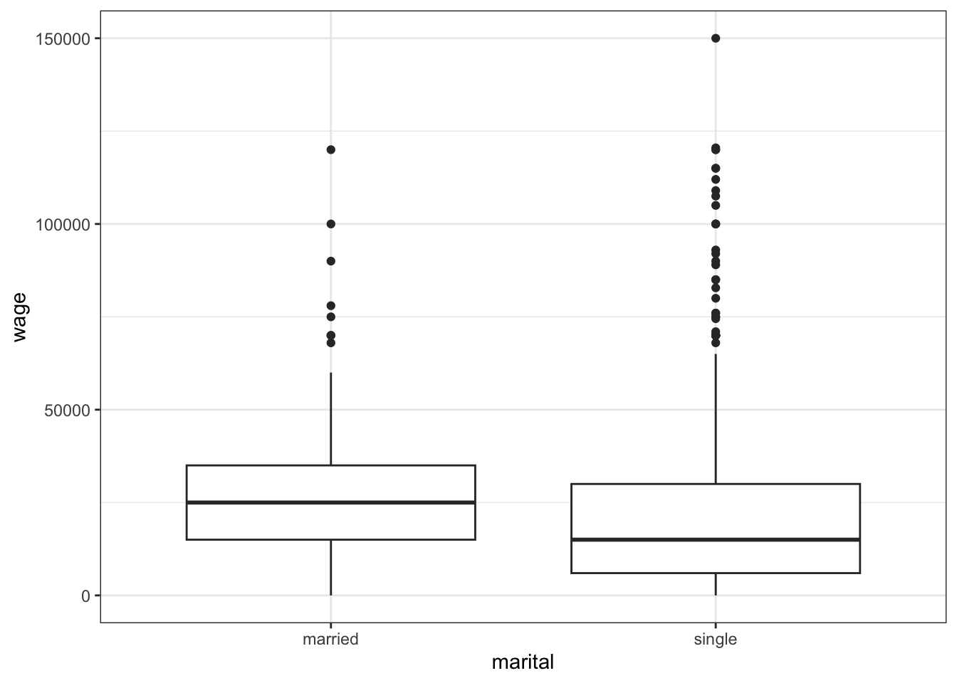
# Model the relationship
wage_model_1 <- lm(wage ~ marital, data = cps)
coef(summary(wage_model_1))
##                Estimate Std. Error   t value     Pr(>|t|)
## (Intercept)   27399.471   1714.496 15.981066 1.849857e-52
## maritalsingle -6596.133   1817.411 -3.629412 2.955178e-04
EXAMPLE 1: Starting a formal hypothesis test
\(H_0\): \(\beta_1 = 0\)
\(H_a\): \(\beta_1 \ne 0\)
EXAMPLE 2: What would we expect under \(H_0\)?
No. It’s more than 3 standard errors away from 0.
# IGNORE THE SYNTAX!!!
# Put OUR sample estimate here
est <- -6596.13

# Put the corresponding standard error here
se <- 1817.41

data.frame(x = 0 + c(-4:4)*se) %>%
  mutate(y = dnorm(x, sd = se)) %>%
  ggplot(aes(x = x)) +
  stat_function(fun = dnorm, args = list(mean = 0, sd = se)) +
  geom_segment(aes(x = x, xend = x, y = 0, yend = y), linetype = "dashed") +
  scale_x_continuous(breaks = c(-4:4)*se) +
  geom_vline(xintercept = est, color = "blue") +
labs(y = "density", x = "possible estimates IF H0 were true") 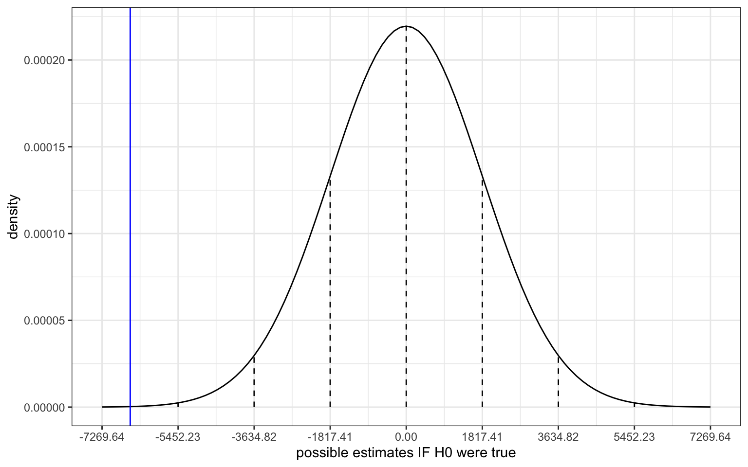
EXAMPLE 3: Test statistic
- .
# By hand
(-6596.133 - 0) / 1817.411
## [1] -3.629412

# This is also reported in the t value column
coef(summary(wage_model_1))
##                Estimate Std. Error   t value     Pr(>|t|)
## (Intercept)   27399.471   1714.496 15.981066 1.849857e-52
## maritalsingle -6596.133   1817.411 -3.629412 2.955178e-04
Our sample estimate of \(\beta_1\) is 3.62 standard errors below the null value of 0.
No – it’s “far” from 0 (3.62 s.e. is far).
EXAMPLE 4: p-value
less than 0.003
Out estimate is more than 3 s.e. from 0. There’s only a 0.003 probability of this happening since the probability of being within 3 s.e. is 0.997.0.000296 (as reported in the
Pr(>|t|)column)
coef(summary(wage_model_1))
##                Estimate Std. Error   t value     Pr(>|t|)
## (Intercept)   27399.471   1714.496 15.981066 1.849857e-52
## maritalsingle -6596.133   1817.411 -3.629412 2.955178e-04
If in fact there were no relationship between wages and marital status in the broader labor force (i.e. \(H_0\) were true), it’s unlikely that we’d have observed such a big wage gap between single and married workers “by chance”. \[P(data | H_0) = \text{prob of observing our data given $H_0$ is true}\]
No – there’s only a small chance we would’ve gotten this data if \(H_0\) were true.
EXAMPLE 5: Conclusion
p-value < 0.05. Thus there’s a statistically significant association between wages and marital status. This agrees with our CI conclusion in Example 1.
Yes, $6596.13 is a lot of money.
EXAMPLE 6: tests for the intercept
- We have statistically significant evidence that the average wage of married workers is non-0.
- We could shift our wage variable by 25000, i.e. model Y = wage - 25000 instead of Y = wage.
Exercise 1: Controlling for age
wage_model_2 <- lm(wage ~ marital + age, data = cps)
coef(summary(wage_model_2))
##                 Estimate Std. Error    t value     Pr(>|t|)
## (Intercept)   -53547.003  5719.1332 -9.3627830 3.484809e-20
## maritalsingle  -1456.015  1714.3082 -0.8493312 3.958595e-01
## age             3483.197   236.4797 14.7293716 2.099717e-45
confint(wage_model_2)
##                    2.5 %     97.5 %
## (Intercept)   -64767.154 -42326.852
## maritalsingle  -4819.252   1907.221
## age             3019.257   3947.138
Part a
\(H_0\): Wage is not associated with marital status when controlling for age.
\(H_a\): Wage is associated with marital status when controlling for age.
Part b
- 95% CI for \(\beta_1\) = (-4819.252, 1907.221)
- test statistic = -0.849
- p-value = 0.396
Part c
When controlling for age, we do not have statistically significant evidence of an association between wage and marital status.
Part d
There is a statistically significant wage gap between single and married workers, but not when considering age.
Part e (OUTSIDE OF CLASS)
- 95% CI: When controlling for age, we’re 95% confident that the average wage of single workers is somewhere between $4810.25 less and $1907.22 more than that of married workers.
- test statistic: Our estimate of the
maritalsingleis only 0.849 standard errors below 0. - p-value: If there were truly no relationship between wage and marital status when controlling for age, there’s a 39.6% (pretty high) chance that we would’ve observed a wage gap as large as we did in our sample.
Exercise 2: Interaction?
Part a
No. It seems like parallel lines would fit within the confidence bands here.
cps %>%
  ggplot(aes(y = wage, x = age, color = marital)) +
  geom_smooth(method = "lm")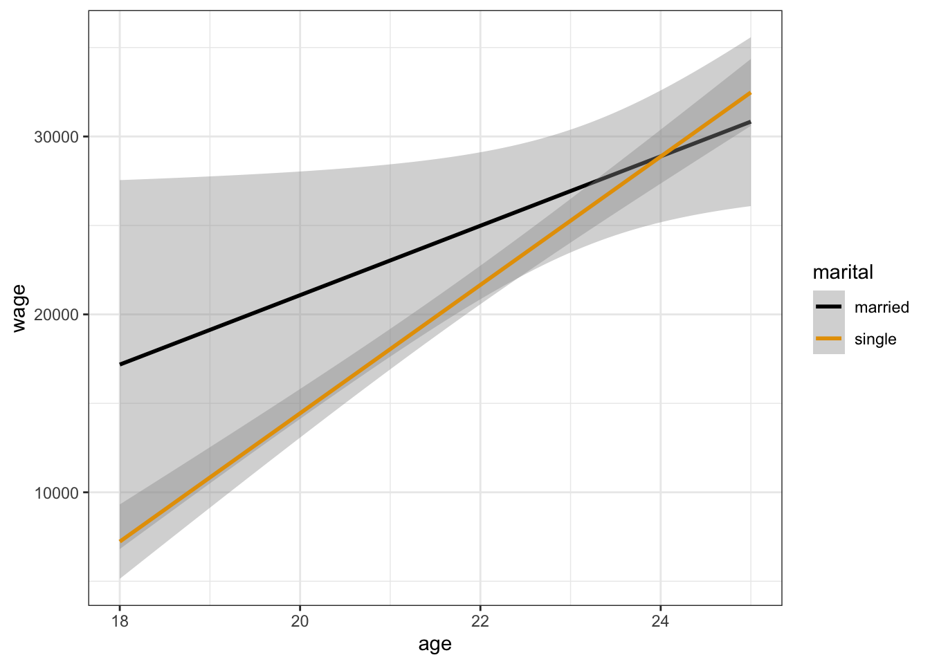
Part b
The interaction term is not significant at the 0.05 level:
wage_model_3 <- lm(wage ~ marital * age, cps)
coef(summary(wage_model_3))
##                     Estimate Std. Error    t value   Pr(>|t|)
## (Intercept)       -17933.067 20129.2894 -0.8908942 0.37315738
## maritalsingle     -39768.593 20834.4327 -1.9087918 0.05651778
## age                 1950.699   863.5021  2.2590547 0.02405167
## maritalsingle:age   1656.498   897.7569  1.8451515 0.06525191
Exercise 3: Spotify Part 1
Part a
Will vary
# Load the data
spotify_small <- read.csv("https://ajohns24.github.io/data/spotify_example_small.csv") %>%
  select(track_artist, track_name, duration_ms, latin_genre) %>%
  mutate(duration = duration_ms / 1000)
nrow(spotify_small)
## [1] 20

spotify_small %>%
  ggplot(aes(y = duration, x = latin_genre)) +
  geom_boxplot()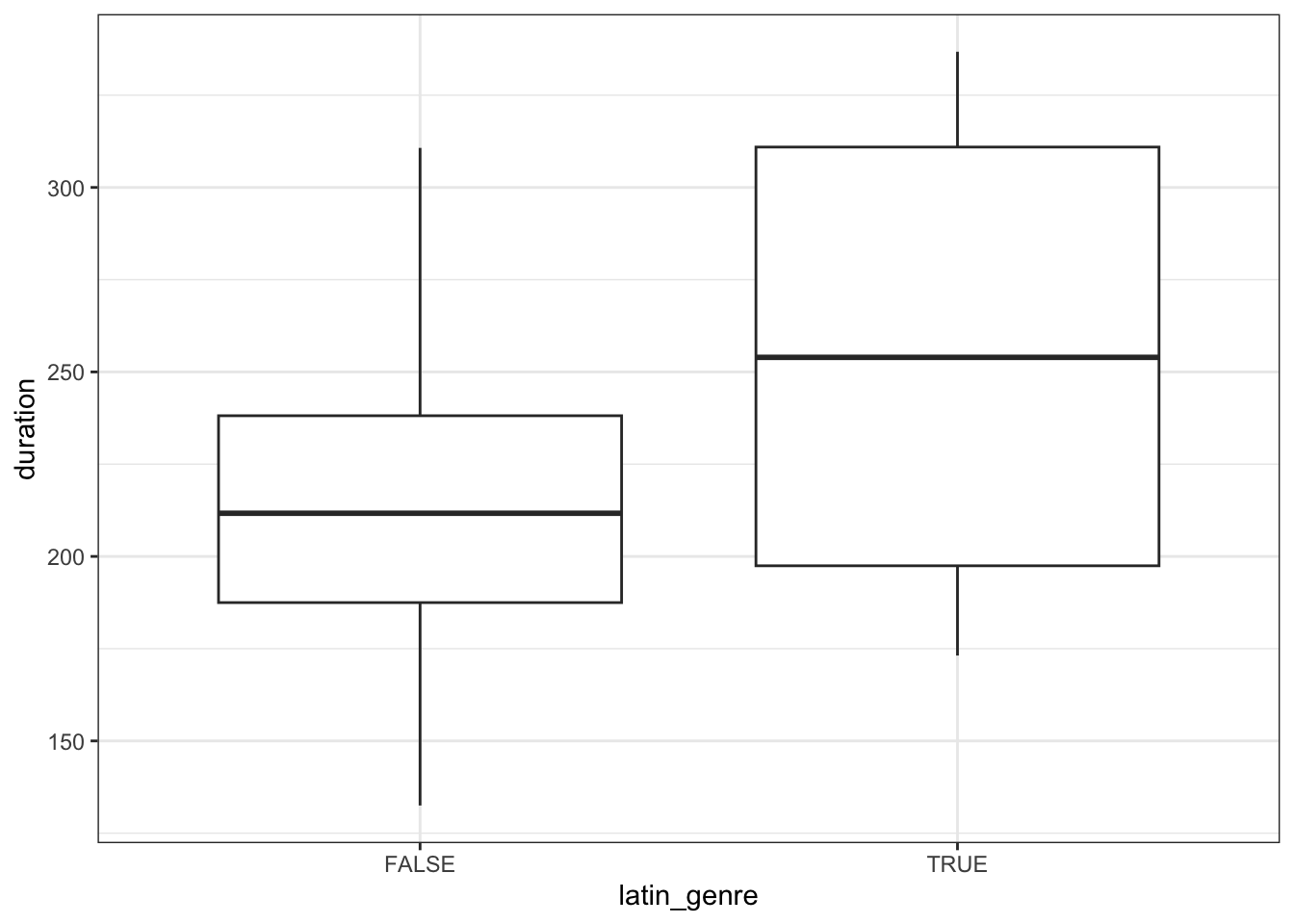
Part b
We estimate that the average length of a latin genre song is 39.5 seconds longer than that of a non-lating genre song. On the scale of time and song lengths, this is a meaningful difference!
spotify_model_1 <- lm(duration ~ latin_genre, spotify_small)
coef(summary(spotify_model_1))
##                  Estimate Std. Error  t value     Pr(>|t|)
## (Intercept)     214.99869   12.97571 16.56932 2.412163e-12
## latin_genreTRUE  39.45606   29.01458  1.35987 1.906619e-01
Part c
The p-value of 0.191 is > 0.05. Thus we do not have statistically significant evidence that the average song duration is different (longer) in the latin genre than in the pop / edm genre.
Exercise 4: Spotify Part 2
spotify_big <- read.csv("https://ajohns24.github.io/data/spotify_example_big.csv") %>%
  select(track_artist, track_name, duration_ms, latin_genre) %>%
  mutate(duration = duration_ms / 1000)
nrow(spotify_big)
## [1] 16216
Part a
Will vary, but these boxplots are very similar, thus it doesn’t seem like there’s a difference.
spotify_big %>%
  ggplot(aes(y = duration, x = latin_genre)) +
  geom_boxplot()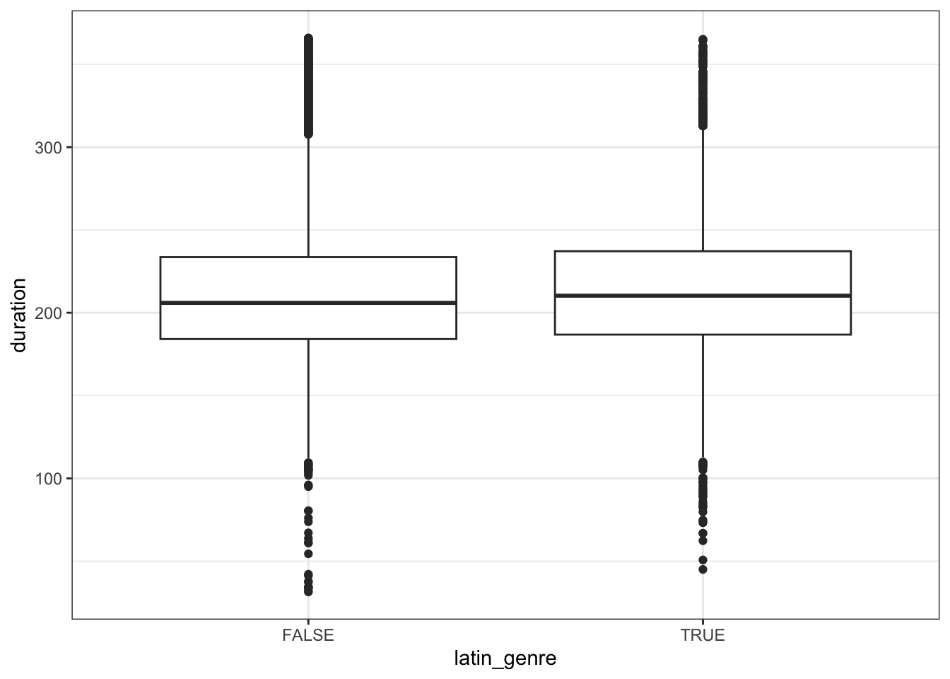
Part b
On average, latin genre songs tend to be 1.56 seconds longer than non-latin songs. This is not a meaningful effect size.
spotify_model_2 <- lm(duration ~ latin_genre, spotify_big)
coef(summary(spotify_model_2))
##                   Estimate Std. Error   t value   Pr(>|t|)
## (Intercept)     212.673908  0.4165491 510.56143 0.00000000
## latin_genreTRUE   1.555355  0.7435700   2.09174 0.03647731
Part c
The p-value of 0.036 is < 0.05. Thus we do have statistically significant evidence that the average song duration is different (longer) in the latin genre than in the pop / edm genre.
Exercise 5: Caution!!
Part a
Large sample size! The more data we have, the smaller our standard errors. Thus the narrower our CIs and the smaller our p-values. Thus the easier it is to establish statistical significance even when the results aren’t practically significant.
Part b
We shouldn’t try to fit a hypothesis test into our narrative. State a significance level and stick with it.
Part c
The more things we test, the more likely something will appear to be “significant” just by chance (even if it’s not). Thus fishing around for significance can lead to misleading conclusions.
Part d
Consider an example that’s closer to life. Will vary.
Exercise 6
mushrooms <- read_csv("https://Mac-STAT.github.io/data/mushrooms.csv") %>%
  mutate(cap_shape = relevel(as.factor(cap_shape), ref = "flat")) %>%
  select(poisonous, cap_shape)

head(mushrooms)
## # A tibble: 6 × 2
##   poisonous cap_shape
##   <lgl>     <fct>
## 1 TRUE      convex
## 2 FALSE     convex
## 3 FALSE     bell
## 4 TRUE      convex
## 5 FALSE     convex
## 6 FALSE     convex
mushrooms %>%
  count(cap_shape)
## # A tibble: 6 × 2
##   cap_shape     n
##   <fct>     <int>
## 1 flat       3152
## 2 bell        452
## 3 conical       4
## 4 convex     3656
## 5 knobbed     828
## 6 sunken       32
Part a
mushroom_mod <- glm(poisonous ~ cap_shape, data = mushrooms, family = "binomial")
coef(summary(mushroom_mod))
Part b
On the log odds scale:
\(H_0\): the log odds that a flat cap mushroom is poisonous are 0
\(H_a\): the log odds that a flat cap mushroom is poisonous are not 0
On the odds scale:
\(H_0\): the odds that a flat cap mushroom is poisonous are 1 (it’s equally likely to be poisonous or edible)
\(H_a\): the odds that a flat cap mushroom is poisonous are not 1 (it’s NOT equally likely to be poisonous or edible)
Part c
The odds of a flat-capped mushroom being poisonous are 0.975. That is, mushrooms with flat caps are very slightly less likely to be poisonous than they are edible.
exp(-0.02538207)
## [1] 0.9749373
Part d
The test statistic is -0.712. This means that the coefficient estimate of interest is 0.712 standard errors away from (specifically, below) the null value of 0 (note that this is on the log-odds scale).
Part e
The p-value for the intercept term is 0.4762. If the null hypothesis were true, the probability of observing a test statistic as or more extreme than |-0.712| is 0.4762. In context: If the odds of being poisonous were 1 (i.e. flat-capped mushrooms were equally likely to be poisonous or edible), there’s a pretty high chance (47.62%) that we would’ve observed an odds ratio as from from 1 as ours was.
Part f
Because the p-value is greater than our significance level of 0.05, we have no evidence to suggest that a flat-capped mushroom is more or less likely to be poisonous.
Exercise 7
Part a
The odds that a conical-capped mushroom is poisonous are 2,172,632 times higher (!) than the odds that a flat-capped mushroom is poisonous. The odds that a knobbed-capped mushroom is poisonous are 2.699 times higher than the odds that a flat-capped mushroom is poisonous.
exp(14.59144985)
exp(0.99296610)
Part b
most worried: conical
least worried: flat
Part c
cap_shapeconical: Our null hypothesis is that the odds ratio between flat-capped and cone-capped mushrooms is 1 (i.e., the odds of a cone-capped mushroom being poisonous are equal to the odds of a flat-capped mushroom being poisonous). If we assume the null hypothesis is true, then the probability of seeing a test statistic as or more extreme than |0.03| is 0.974 (i.e., we are very likely to see a test statistic more extreme than |-0.03| if in fact there were no difference between flat-capped and cone-cap mushrooms in odds of being poisonous). Because the p-value is far above our significance level of 0.05, we do not have evidence that the odds of a cone-capped mushroom being poisonous differ from the odds of a flat-capped mushroom being poisonous.
cap_shapeknobbed: Our null hypothesis is that the odds ratio between flat-capped and knob-capped mushrooms is 1 (i.e., the odds of a knob-capped mushroom being poisonous are equal to the odds of a flat-capped mushroom being poisonous). If we assume the null hypothesis is true, then the probability of seeing a test statistic as or more extreme than |11.60| is 3.91e-31. Because the p-value is far below our significance level of 0.05, we take this as strong evidence that knob-capped mushrooms are much more likely to be poisonous than flat-capped mushrooms.
Part d
Only considering coefficient estimates, then conical-shaped caps seem the most dangerous – but they’re not significantly different than flat-shaped mushrooms. Only considering p-values, then knob-shaped caps have the strongest evidence that they are more likely to be poisonous than flat-shaped mushrooms.
Part e
Personally, I’d stick with sunken-shaped caps for eating. Even though our model suggests there’s no evidence to believe they are less likely to be poisonous, 0 out of 32 in the sample are poisonous, which seems like the least risky choice. However, I’d tend to avoid the knob-capped mushrooms more than the conical-capped mushrooms. Even though the latter are all poisonous in the sample, there were only 4 observations, so it’s possible that due to sampling variation, the odds of being poisonous for cone-capped mushrooms is lower than that of knob-capped mushrooms (where we have many more observations).
mushrooms %>%
  count(cap_shape, poisonous)
## # A tibble: 10 × 3
##    cap_shape poisonous     n
##    <fct>     <lgl>     <int>
##  1 flat      FALSE      1596
##  2 flat      TRUE       1556
##  3 bell      FALSE       404
##  4 bell      TRUE         48
##  5 conical   TRUE          4
##  6 convex    FALSE      1948
##  7 convex    TRUE       1708
##  8 knobbed   FALSE       228
##  9 knobbed   TRUE        600
## 10 sunken    FALSE        32
Exercise 8
fish <- read_csv("https://Mac-STAT.github.io/data/Mercury.csv")
head(fish)
## # A tibble: 6 × 5
##   River  Station Length Weight Concen
##   <chr>    <dbl>  <dbl>  <dbl>  <dbl>
## 1 Lumber       0   47     1616   1.6
## 2 Lumber       0   48.7   1862   1.5
## 3 Lumber       0   55.7   2855   1.7
## 4 Lumber       0   45.2   1199   0.73
## 5 Lumber       0   44.7   1320   0.56
## 6 Lumber       0   43.8   1225   0.51
Part a
mod_fish1 <- lm(Concen ~ Length + River, fish)
summary(mod_fish1)
##
## Call:
## lm(formula = Concen ~ Length + River, data = fish)
##
## Residuals:
##      Min       1Q   Median       3Q      Max
## -1.19298 -0.36849 -0.07677  0.30905  1.84773
##
## Coefficients:
##               Estimate Std. Error t value Pr(>|t|)
## (Intercept)  -1.194229   0.216287  -5.521 1.26e-07 ***
## Length        0.057657   0.005213  11.061  < 2e-16 ***
## RiverWacamaw  0.142027   0.089496   1.587    0.114
## ---
## Signif. codes:  0 '***' 0.001 '**' 0.01 '*' 0.05 '.' 0.1 ' ' 1
##
## Residual standard error: 0.5779 on 168 degrees of freedom
## Multiple R-squared:  0.431,  Adjusted R-squared:  0.4243
## F-statistic: 63.63 on 2 and 168 DF,  p-value: < 2.2e-16
Part b
coefficient: Holding fish length constant, we estimate the average mercury concentration among fish in the Wacamaw River to be 0.14ppm higher than fish in the Lumber River.
Test statistic: The estimate we observe (0.14) is 1.587 standard errors higher than the null value of a 0ppm difference in mercury concentration.
p-value: Assuming the null hypothesis is true and there is no actual difference in mercury concentration among the two fish populations (adjusting for fish length), the probability of observing a test statistic as or more extreme than |1.587| is 0.114. Because 0.114 > 0.05, we do not have sufficient evidence to reject the null hypothesis, and conclude that the average mercury concentration does not differ between the two rivers.
Part c
fish %>%
  ggplot(aes(x = Length, y = Concen, colour = River)) +
  geom_point()+
  geom_smooth(method = "lm")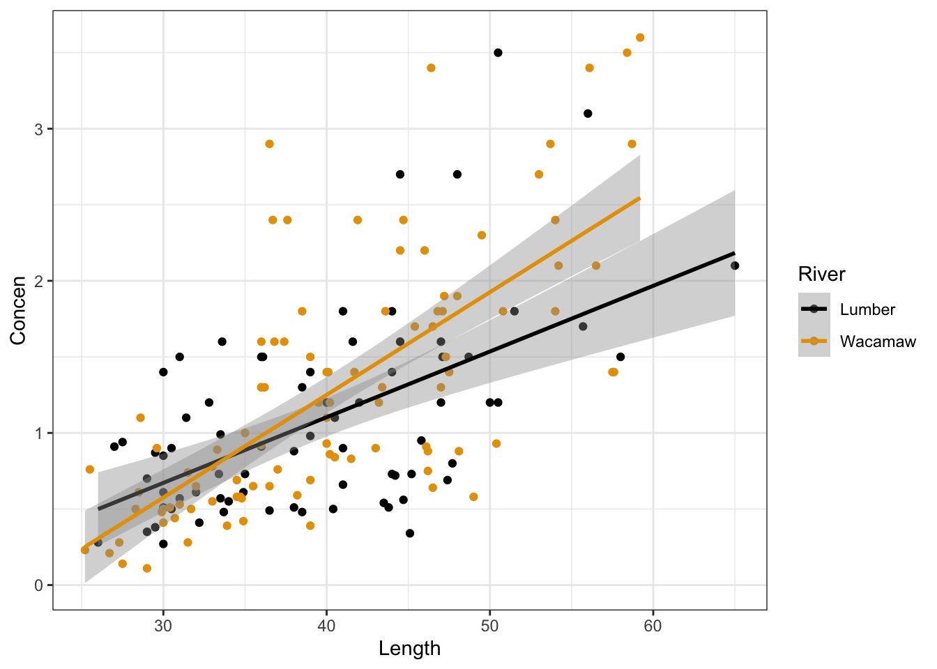
mod_fish2 <- lm(Concen ~ Length * River, fish)
summary(mod_fish2)
##
## Call:
## lm(formula = Concen ~ Length * River, data = fish)
##
## Residuals:
##      Min       1Q   Median       3Q      Max
## -1.27784 -0.35402 -0.08314  0.30650  1.94304
##
## Coefficients:
##                      Estimate Std. Error t value Pr(>|t|)
## (Intercept)         -0.623875   0.325576  -1.916   0.0570 .
## Length               0.043185   0.008085   5.341 2.99e-07 ***
## RiverWacamaw        -0.826291   0.426529  -1.937   0.0544 .
## Length:RiverWacamaw  0.024326   0.010483   2.321   0.0215 *
## ---
## Signif. codes:  0 '***' 0.001 '**' 0.01 '*' 0.05 '.' 0.1 ' ' 1
##
## Residual standard error: 0.5705 on 167 degrees of freedom
## Multiple R-squared:  0.4488, Adjusted R-squared:  0.4389
## F-statistic: 45.33 on 3 and 167 DF,  p-value: < 2.2e-16
Part d
coefficient: First, we interpret the Length coefficient–that is, among fish in the Lumber river, we expect that a 1cm increase in length is associated with a 0.043ppm increase in mercury concentration. The interaction coefficient tells us the expected change in that relationship when considering fish in the Wacamaw River instead: we expect an additional 0.024ppm increase in mercury concentration associated with a 1cm increase in length (i.e., in the Wacamaw River, we expect mercury concentration to increase by 0.067ppm per 1cm increase in fish length).
Test statistic: The estimate we observe (0.024326) is 2.321 standard errors higher than the null value of zero.
p-value: Assuming the null hypothesis is true and there is no difference in the relationship between fish length and mercury between the 2 rivers, the probability of observing a test statistic as or more extreme than |2.321| is 0.02. Because 0.02 < 0.05, we take this as evidence to reject the null hypothesis, and conclude that the effect of fish length on mercury concentration does differ slightly between the two rivers.
Part e
coefficient: Visually, the RiverWacamaw coefficient represents the difference in the y-intercepts for the best fit lines for the Lumber and Wacamaw Rivers in the part d plot. Interpretation: Among fish that are 0cm long, average fish mercury concentrations are 0.826ppm lower in the Wacamaw River than in the Lumber River.
Test statistic: The estimate we observe (-0.826291) is 1.937 standard errors lower than the null value of 0.
p-value: Assuming the null hypothesis is true, the probability of observing a test statistic as or more extreme than |-1.937| is 0.0544. Because 0.0544 > 0.05, we do not have evidence to reject the null.
Part f (CHALLENGE)
p-value = 0.0544/2 = 0.0272 (we divide the “two-tailed” p-value in half to obtain the p-value for a “one-tailed” test)
It is possible that the researchers had a particular reason or incentive to publish evidence in support of their hypothesis (some potential reasons are that scientific journals are generally less interested in publishing results, a financial conflict of interests, or favoring a pet hypothesis). They could have first looked at the results of a “two-tailed” statistical test and since the p-value is very close to the traditional significance threshold of 0.05, come up with a post-hoc rationalization to perform a hypothesis test resulting in a “statistically significant” p-value. This unethical practice is known in the field as “p-hacking.”