8 Multiple regression principles

Announcements etc

SETTLING IN

Put away cell phones (like in your backpack, not face down on your table).
Sit in your new assigned groups. Meet one another!
Download “08-mlr-principles-notes.qmd”, open it in RStudio, and save it in the “Activities” sub-folder of the “STAT 155” folder.
MSCS events
- Thursday, 11:15-11:45am: MSCS coffee break
- Thursday, 3:00-4:30pm: Math problem solving. All experience levels welcome!

WRAPPING UP

Upcoming due dates:
- This week
  - Thursday = CP 7
    - Why use CPs?! This is important prep for class, just like another class that might assign readings + reading reflections.
- Next week
  - Tuesday = PP 3 & CP 8
  - Thursday = CP 9 & Quiz 1 revisions by the start of class. Please review the syllabus for details.
Continued reminders
- Start PP 3 today if you haven’t already!
- If you don’t finish an activity during class, you should complete it outside of class and check the online solutions! This is important prep for moving on to the next topic.
- Study on an ongoing basis, not just right before quizzes!
Quiz 3
If you believe you have extenuating, unavoidable circumstances that will prevent you from taking Quiz 3 at the scheduled time (or make it extremely challenging), email me ASAP.

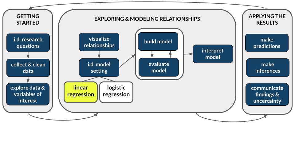
Learning goals

We’re still talking about linear regression models! But now, we have multiple predictors in our models. Accordingly, the plots and models of the relationships of interest can get complicated. Though there are no recipes for this process, there are some guiding principles that assist in long-term retention, deeper understanding, and the ability to generalize our tools in new settings. Today we’ll explore some general principles for…

incorporating additional quantitative or categorical predictors in a visualization
how additional quantitative or categorical predictors impact the physical representation of a model
interpreting quantitative or categorical coefficients in a multiple regression model

Additional resources

Required video

Multivariate modeling principles (slides)

Optional

The below videos provide extra examples for interpreting multiple linear regression models. You’re encouraged to watch them after today’s activity.

Interpreting multivariate models (Part I) and Part II (slides)

Warm-up

Let’s revisit the bikeshare data:

# Load packages & import data
library(tidyverse)
bikes <- read_csv("https://mac-stat.github.io/data/bikeshare.csv") %>% 
  rename(rides = riders_registered)

# Check out the data
head(bikes)

Our goal is to explore how registered ridership varies from day to day. To this end, we’ll build various multiple linear regression models of rides by different combinations of the possible predictors.

EXAMPLE 1: Visualization review

Let’s explore the relationship of rides with windspeed (quantitative) and weekend status (categorical):

bikes %>% 
  select(rides, windspeed, weekend) %>% 
  head()

Write a model statement for this regression model.

E[rides | windspeed, weekend] = \(\beta_0\) + \(\beta_1\) windspeed + \(\beta_2\) ___

Construct and discuss a plot of the relationship between these 3 variables. NOTE: Make sure that your description addresses all variables here, as well as the strength of the overall relationship.

# Plot of rides vs windspeed & weekend
# Include a representation of the linear regression model
# PRO TIP: Start with a plot of rides by windspeed, then modify it
bikes %>% 
  ggplot(aes(y = rides, x = windspeed)) + 
  geom___() + 
  geom_smooth(method = "lm", se = FALSE)

EXAMPLE 2: Model review

Let’s build the linear regression model of this relationship:

bike_model_1 <- lm(rides ~ windspeed + weekend, data = bikes)
summary(bike_model_1)

Thus estimated model formula is:

E[rides | windspeed, weekend] = 4738.38 - 63.97 windspeed - 925.16 weekendTRUE

This model formula is represented by 2 lines, one corresponding to weekends and the other to weekdays. Simplify the model formula above for weekdays and weekends:

weekdays: rides = ___ - ___ windspeed

weekends: rides = ___ - ___ windspeed

# Record any calculations here

EXAMPLE 3: Coefficient interpretation review

The intercept coefficient, 4738.38, represents the intercept of the sub-model for weekdays, the reference category. What’s its contextual interpretation?
The windspeed coefficient, -63.97, represents the shared slope of the weekend and weekday sub-models. What’s its contextual interpretation?
The weekendTRUE coefficient, -925.16, represents the change in intercept for the weekend vs weekday sub-model. What’s its contextual interpretation?

Interpreting MLR coefficients (2 predictors)

Consider a multiple linear regression model with 2 predictors:

\[E[Y | X_1, X_2] = \beta_0 + \beta_1 X_1 + \beta_2 X_2\]

Then

\(\beta_0\) (“beta 0”) = expected value of \(Y\) when \(X_1\) and \(X_2\) are both 0, ie. when all quantitative predictors are set to 0 and the categorical predictors are set to their reference levels.
\(\beta_1\) (“beta 1”) = change in the expected value of \(Y\) for two cases whose values of \(X_1\) differ by 1 but who are identical in terms of \(X_2\).

OPTIONAL Math Box: Fitting multiple linear regression models

Consider a multiple linear regression model with \(p\) predictors:

\[E[Y|X_1,X_2,...,X_p] = \beta_0 + \beta_1 X_1 + \beta_2 X_2 + ... + \beta_p X_p\]

We use the least squares criterion to estimate \((\beta_0, \beta_1, ..., \beta_p)\), i.e. we pick the coefficients minimize the sum of squared residuals. Just as with simple linear regression, we can write out a formula for these least square estimates. But for multiple linear regression, this requires linear algebra.

Suppose we have \(n\) data points. Using matrix notation, we can collect our observed response values into a vector \(Y\), our predictor values into a matrix \(X\), and our regression coefficients into a vector \(\beta\). The column of 1s in \(X\) reflects our model’s inclusion of an intercept:

\[Y = \left(\begin{array}{c} Y_1 \\ Y_2 \\ \vdots \\ Y_n \end{array} \right) \;\;\;\; \text{ and } \;\;\;\; X = \left(\begin{array}{ccccc} 1 & X_{11} & X_{12} & \cdots & X_{1p} \\ 1 & X_{21} & X_{22} & \cdots & X_{2p} \\ \vdots & \vdots & \vdots & \cdots & \vdots \\ 1 & X_{n1} & X_{n2} & \cdots & X_{np} \\ \end{array} \right) \;\;\;\; \text{ and } \;\;\;\; \beta = \left(\begin{array}{c} \beta_0 \\ \beta_1 \\ \vdots \\ \beta_p \end{array} \right)\]

Then we can express the model \(E[Y_i|X_{i1}, X_{i2},...,X_{ip}] = \beta_0 + \beta_1 X_{i1} + \cdots + \beta_p X_{ip}\) for \(i \in \{1,...,n\}\) as:

\[E[Y|X] = X\beta\] Further, let \(\hat{\beta}\) denote the vector of sample estimated \(\beta\) and \(\hat{Y}\) denote the vector of predictions / model values:

\[\hat{Y} = X \hat{\beta}\]

Thus the sum of squared residuals is

\[\sum_{i=1}^n (Y_i - \hat{Y}_i)^2 = (Y - \hat{Y})^T(Y - \hat{Y}) = (Y - X \hat{\beta})^T(Y - X \hat{\beta})\]

and the following formula for sample coefficients \(\hat{\beta}\) are the least squares estimates of \(\beta\), i.e. they minimize the sum of squared residuals:

\[\hat{\beta} = (X^TX)^{-1}X^TY\]

Exercises

Thus far, we’ve explored a couple examples of multiple regression models that have 2 predictors, 1 quantitative and 1 categorical. Let’s explore what happens when both predictors are categorical or both are quantitative!

Exercise 1: 2 categorical predictors – visualization

Let’s explore the relationship of rides with 2 categorical predictors, weekend status and season. The below code plots rides vs just season. Modify this code to also include information about weekend. HINT: Remember the visualization principle that additional categorical predictors require some sort of grouping mechanism that distinguishes between the groups.

# Modify this code to plot rides vs season AND weekend
bikes %>% 
  ggplot(aes(y = rides, x = season)) + 
  geom_boxplot()

Exercise 2: follow-up

Part a

Describe, in words, the relationship of ridership with season & weekend status. In doing so, address the following:

No matter the weekend status, how is ridership associated with season?
No matter the season, how is ridership associated with weekend status?
Does the overall relationship of ridership with season & weekend status appear to be strong?

Part b

A model of rides by season alone would be represented by only 4 expected outcomes, 1 for each season. Considering this and the plot above, how do you anticipate a model of rides by season and weekend status will be represented?

2 lines, 1 for each weekend status
8 lines, 1 for each possible combination of season & weekend
2 expected outcomes, 1 for each weekend status
8 expected outcomes, 1 for each possible combination of season & weekend

Exercise 3: 2 categorical predictors – modeling

Build the multiple regression model of rides vs season and weekend:

bike_model_2 <- lm(rides ~ weekend + season, bikes)
summary(bike_model_2)

Thus the estimated model formula is:

E[rides | weekend, season] = 4260.45 - 912.33 weekendTRUE - 116.38 seasonspring + 438.44 seasonsummer - 1719.06 seasonwinter

Part a

Use this model to make the following predictions:

# predicted ridership on a fall weekday
4260.45 - 912.33*___ - 116.38*___  + 438.44*___ - 1719.06*___

# predicted ridership on a winter weekday    
4260.45 - 912.33*___ - 116.38*___  + 438.44*___ - 1719.06*___

# predicted ridership on a winter weekend day
4260.45 - 912.33*___ - 116.38*___  + 438.44*___ - 1719.06*___

Using the calculations in the chunk above, calculate the differences between various predictions:

# diff in predicted ridership on a winter weekday vs a fall weekday
# (that is, the diff btwn 2 days that are at the same time of week but DIFFERENT seasons)
# WHERE HAVE YOU OBSERVED THIS NUMBER BEFORE?!
___ - ___

# diff in predicted ridership on a winter weekend vs a winter weekday
# (that is, the diff btwn 2 days that are in the same season but DIFFERENT times of the week)
# WHERE HAVE YOU OBSERVED THIS NUMBER BEFORE?!
___ - ___

Part b

We only made 3 predictions here. In general there are 8 possible predictions: 2 weekend categories x 4 season categories. Is this consistent with your intuition in the previous exercise?

Exercise 4: 2 categorical predictors – interpret the model

Use your above predictions and visualization to fill in the below interpretations of the model coefficients. Hint: What is the consequence of plugging in 0 or 1 for the different weekend and season categories?

Interpreting 4260: On average, there are 4260 riders on (weekdays/weekends) during the (fall/spring/summer/winter), i.e. when all predictors are “0”
Interpreting -912: On average, in any season, there are 912 (more/fewer) riders on weekends than on ___.
Interpreting -1719: On average, on both weekdays and weekends, we expect there to be 1719 (more/fewer) riders in winter than in ___.

Exercise 5: 2 quantitative predictors – visualization

Next, consider the relationship of rides with 2 quantitative predictors: windspeed and temp_feel. Check out the plot of this relationship below which reflects the visualization principle that quantitative variables require some sort of numerical scaling mechanism – rides and windspeed get numerical axes, and temp_feel gets a color scale:

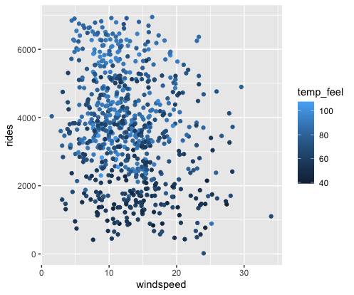
Modify the code below to recreate this plot:

bikes %>%
  ggplot(aes(___)) +
  geom_point()

OPTIONAL: Check out this interactive plot which allows us to explore this point cloud in 3D.

library(plotly)
bikes %>% 
  plot_ly(x = ~windspeed, y = ~temp_feel, z = ~rides, 
          type = "scatter3d", 
          mode = "markers",
          marker = list(size = 5, color = ~rides, colorscale = "Viridis"))

Exercise 6: follow-up

Describe (in words) the relationship of ridership with windspeed & temperature. Make sure to comment on all 3 variables, strength of the relationship, and any outliers (if relevant).

Exercise 7: 2 quantitative predictors – modeling

Let’s build the multiple regression model of rides vs windspeed and temp_feel:

bike_model_3 <- lm(rides ~ windspeed + temp_feel, data = bikes)
summary(bike_model_3)

Thus the estimated model formula is:

E[rides | windspeed, temp_feel] = -24.06 - 36.54 windspeed + 55.52 temp_feel

Part a

Interpret the intercept coefficient, -24.06, in context.

Part b

Interpret the windspeed coefficient, -36.54, in context.

Part c

Interpret the temp_feel coefficient, 55.52, in context.

Exercise 8: Which model is “best”?

We’ve now observed 3 different models of ridership, each having 2 predictors. The R-squared values of these models, along with those of the simple linear regression models with each predictor alone, are summarized below.

model	predictors	R-squared
`bike_model_1`	`windspeed` & `weekend`	0.119
`bike_model_2`	`weekend` & `season`	0.349
`bike_model_3`	`windspeed` & `temp_feel`	0.310
`bike_model_4`	`windspeed`	0.047
`bike_model_5`	`temp_feel`	0.296
`bike_model_6`	`weekend`	0.074
`bike_model_7`	`season`	0.279

Part a

Which model does the best job of explaining the variability in ridership from day to day?

Part b

If you could only pick one predictor, which would it be?

Part c

What happens to R-squared when we add a second predictor to our model, and why does this make sense? For example, how does the R-squared for model 1 (with both windspeed and weekend) compare to those of model 4 (only windspeed) and model 6 (only weekend)?

Part d

Are 2 predictors always better than 1? Provide evidence for your answer and explain why this makes sense.

Exercise 9: Principles of interpretation

These exercises have confirmed the principles behind interpreting model coefficients, summarized below. Review and confirm that these make sense.

Interpretating MLR coefficients (2+ predictors)

Consider a multiple linear regression model:

\[E[Y | X_1, X_2, ..., X_p] = \beta_0 + \beta_1 X_1 + \beta_2 X_2 + ... + \beta_p X_p\]

\(\beta_0\) (“beta 0”) = expected value of \(Y\) when the \(X_i\) are all 0, ie. when all quantitative predictors are set to 0 and the categorical predictors are set to their reference levels.
\(\beta_1\) (“beta 1”) = change in the expected value of \(Y\) for two cases whose values of \(X_1\) differ by 1 but who are identical in terms of all other \(X\):
- If \(X_1\) is quantitative, \(\beta_1\) describes the change in the expected value of \(Y\) associated with a 1-unit increase in \(X_1\), while at a fixed set of the other \(X\).
- If \(X_1\) represents a category of a categorical variable, \(\beta_1\) describes the change in the expected value of \(Y\) between this category and the reference category, while at a fixed set of the other \(X\).

Exercise 10: Extra Practice 1

The following exercises provide extra practice. Consider the relationship of rides vs weekend and weather_cat.

Construct a visualization of this relationship.
Construct a model of this relationship.
Interpret the first 3 model coefficients.

Exercise 11: Extra Practice 2

Consider the relationship of rides vs temp_feel and humidity.

Construct a visualization of this relationship.
Construct a model of this relationship.
Interpret the first 3 model coefficients.

Exercise 12: Extra Practice 3

Consider the relationship of rides vs temp_feel and weather_cat.

Construct a visualization of this relationship.
Construct a model of this relationship.
Interpret the first 3 model coefficients.

Exercise 13: Optional CHALLENGE

We’ve explored models with 2 predictors. What about 3 predictors?! Consider the relationship of rides vs temp_feel, humidity, AND weekend.

Construct a visualization of this relationship.
Construct a model of this relationship.
Interpret each model coefficient.

Exercise 14: Explore more examples

Outside of class, check out the below videos that include extra examples:

Interpreting multivariate models (Part I) and Part II (slides)

Solutions

EXAMPLE 1: Visualization review

E[rides | windspeed, weekend] = \(\beta_0\) + \(\beta_1\) windspeed + \(\beta_2\) weekendTRUE

On both weekends and weekdays, there’s a week negative association between ridership and windspeed – ridership tends to decrease as windspeed increase.
At any windspeed, there tend to be fewer riders on weekends.
This relationship seems relatively weak. There’s a lot of variability from the model within each weekend group, and quite a bit of overlap between these 2 groups.

bikes %>% 
  ggplot(aes(y = rides, x = windspeed, color = weekend)) + 
  geom_point() + 
  geom_smooth(method = "lm", se = FALSE)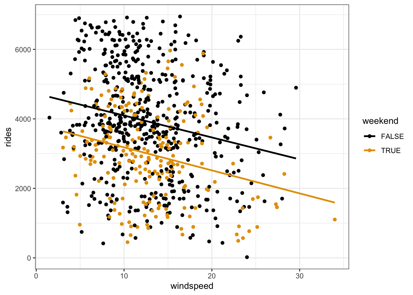

EXAMPLE 2: Model review

weekdays: rides = 4738.38 - 63.97 windspeed

weekends: rides = 4738.38 - 63.97 windspeed - 925.16 = 3813.22 - 63.97 windspeed

EXAMPLE 3: Coefficient interpretation review

On average, there are 4738 riders on weekdays with 0 windspeed.
On both weekends and weekdays, a 1mph increase in windspeed is associated with a 64 rider decrease in average ridership.
At any windspeed, the average ridership is 925 lower on weekends than week days.

Exercise 1: 2 categorical predictors – visualization

bikes %>% 
  ggplot(aes(y = rides, x = season, color = weekend)) + 
  geom_boxplot()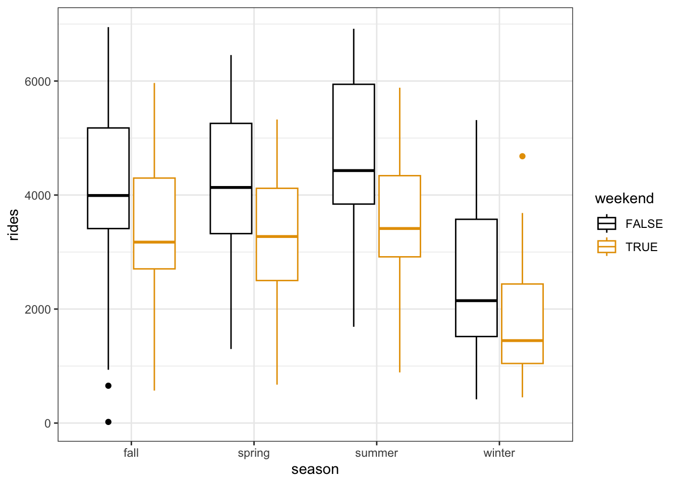

bikes %>% 
  ggplot(aes(y = rides, x = season, fill = weekend)) + 
  geom_boxplot()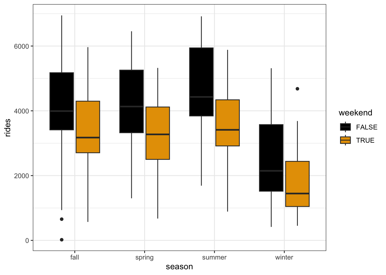

Exercise 2: follow-up

Ridership tends to be lower on weekends (not matter the season). And no matter the weekend status, ridership tends to be highest in summer and lowest in winter. These relationships are relatively strong, as signified by the small overlap in the weekend / weekday boxes and the summer / winter boxes.
8 expected outcomes

Exercise 3: 2 categorical predictors – modeling

# predicted ridership on a fall weekday
4260.45 - 912.33*0 - 116.38*0 + 438.44*0 - 1719.06*0
## [1] 4260.45

# predicted ridership on a winter weekday    
4260.45 - 912.33*0 - 116.38*0 + 438.44*0 - 1719.06*1
## [1] 2541.39

# predicted ridership on a winter weekend day
4260.45 - 912.33*1 - 116.38*0 + 438.44*0 - 1719.06*1
## [1] 1629.06

# diff in predicted ridership on a winter weekday vs a fall weekday
# (that is, the diff btwn 2 days that are at the same time of week but DIFFERENT seasons)
# THIS IS THE VALUE OF THE seasonwinter COEF
2541.39 - 4260.45
## [1] -1719.06

# diff in predicted ridership on a winter weekend vs a winter weekday
# (that is, the diff btwn 2 days that are in the same season but DIFFERENT times of the week)
# THIS IS THE VALUE OF THE weekendTRUE COEF
1629.06 - 2541.39
## [1] -912.33

will vary

Exercise 4: 2 categorical predictors – interpret the model

On average, there are 4260 riders on weekdays during the fall.
On average, in any season, there are 912 fewer riders on weekends than on weekdays.
On average, on both weekdays and weekends, there are 1719 fewer riders in winter than in fall.

Exercise 5: 2 quantitative predictors – visualization

bikes %>% 
  ggplot(aes(y = rides, x = windspeed, color = temp_feel)) + 
  geom_point()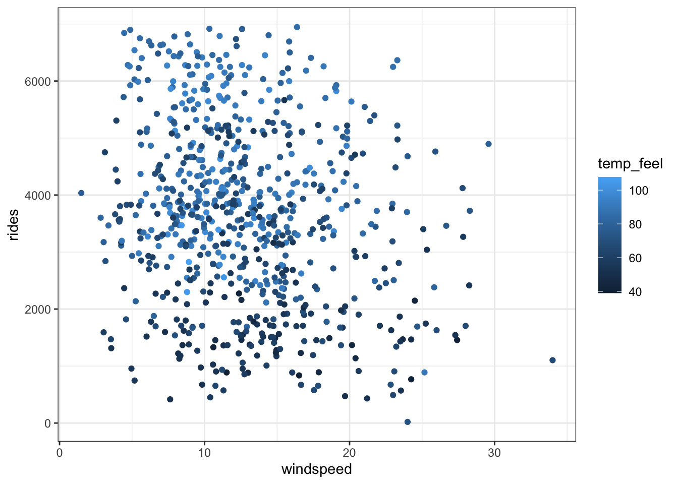

Exercise 6: follow-up

Ridership tends to increase with temperature (no matter the windspeed) and decrease with windspeed (no matter the temperature). The relationship is pretty strong. There’s one possible outlier on a day with high temperature and high windspeed, but relatively few rides.

8.1 Exercise 7: 2 quantitative predictors – modeling

-24.06 = average ridership on days with 0 windspeed and a 0 degree temperature. (Note: this is a correct interpretation, even though it doesn’t make conceptual sense! The model doesn’t know that ridership can’t be negative!)
At any temperature, a 1mph increase in windspeed is associated with a 37 rider decrease in average ridership.
At any windspeed, a 1 degree increase in temperature is associated with a 56 rider increase in average ridership.

Exercise 8: Which model is “best”?

model 2
temperature
R-squared increases (our model is stronger when we include another predictor)
nope. model 1 (with windspeed and weekend) has a lower R-squared than model 5 (with only temperature)

Exercise 10: Extra Practice 1

bikes %>% 
  ggplot(aes(y = rides, x = weekend, fill = weather_cat)) + 
  geom_boxplot()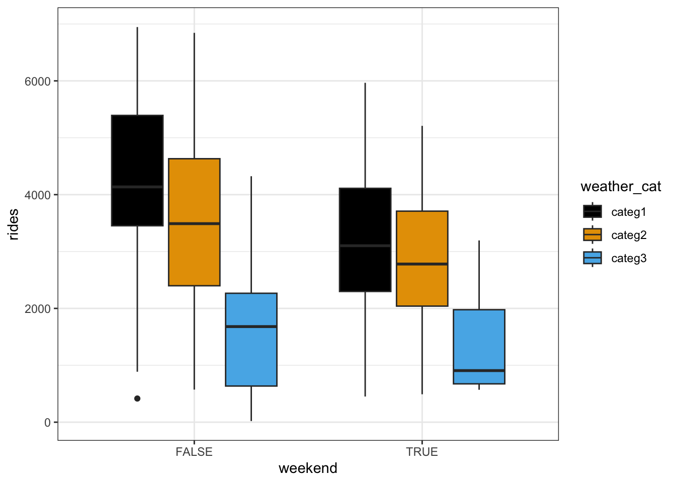


new_model_1 <- lm(rides ~ weekend + weather_cat, bikes)
summary(new_model_1)
## 
## Call:
## lm(formula = rides ~ weekend + weather_cat, data = bikes)
## 
## Residuals:
##     Min      1Q  Median      3Q     Max 
## -3795.9  -882.4   -73.9  1072.2  3241.0 
## 
## Coefficients:
##                   Estimate Std. Error t value Pr(>|t|)    
## (Intercept)        4211.87      75.55  55.752  < 2e-16 ***
## weekendTRUE        -982.21     117.25  -8.377 2.79e-16 ***
## weather_catcateg2  -608.86     113.00  -5.388 9.63e-08 ***
## weather_catcateg3 -2360.20     319.72  -7.382 4.27e-13 ***
## ---
## Signif. codes:  0 '***' 0.001 '**' 0.01 '*' 0.05 '.' 0.1 ' ' 1
## 
## Residual standard error: 1433 on 727 degrees of freedom
## Multiple R-squared:  0.1605, Adjusted R-squared:  0.157 
## F-statistic: 46.31 on 3 and 727 DF,  p-value: < 2.2e-16

The average ridership on a weekday with nice weather (categ1) is 4212 rides.
On days with the same weather, the average ridership is 982 less on a weekend than on a weekday.
On any day of the week, the average ridership is 609 less on dreary days than on nice days.

Exercise 11: Extra Practice 2

bikes %>% 
  ggplot(aes(y = rides, x = temp_feel, color = humidity)) + 
  geom_point()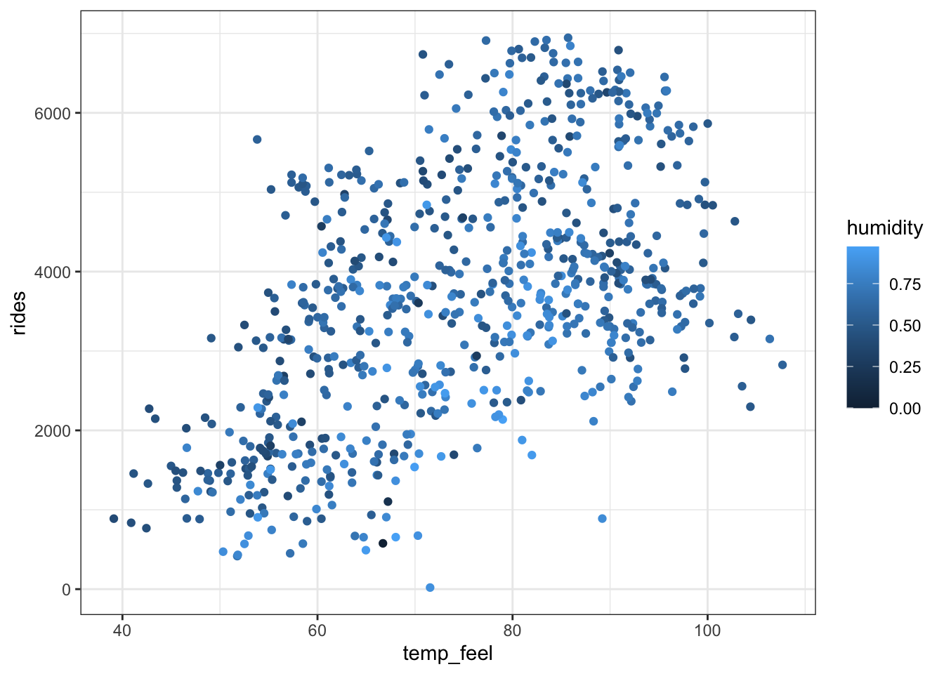


new_model_2 <- lm(rides ~ temp_feel + humidity, bikes)
summary(new_model_2)
## 
## Call:
## lm(formula = rides ~ temp_feel + humidity, data = bikes)
## 
## Residuals:
##     Min      1Q  Median      3Q     Max 
## -3770.3  -972.7  -150.6   967.7  3163.8 
## 
## Coefficients:
##              Estimate Std. Error t value Pr(>|t|)    
## (Intercept)   315.837    303.777   1.040    0.299    
## temp_feel      60.433      3.272  18.468  < 2e-16 ***
## humidity    -1868.994    336.964  -5.547 4.08e-08 ***
## ---
## Signif. codes:  0 '***' 0.001 '**' 0.01 '*' 0.05 '.' 0.1 ' ' 1
## 
## Residual standard error: 1284 on 728 degrees of freedom
## Multiple R-squared:  0.3247, Adjusted R-squared:  0.3228 
## F-statistic:   175 on 2 and 728 DF,  p-value: < 2.2e-16

On average, there are 316 riders on days with 0 humidity that feel like 0 degrees.
At any humidity, a 1 degree increase in ridership is associated with a 60 ride increase in average ridership.
At any temperature, a 1 percentage point increase in humidity (i.e. a 0.1 increase in humidity) is associated with a 187 decrease in average ridership.

Exercise 12: Extra Practice 3

new_model_3 <- lm(rides ~ temp_feel + weather_cat, bikes)
summary(new_model_3)
## 
## Call:
## lm(formula = rides ~ temp_feel + weather_cat, data = bikes)
## 
## Residuals:
##     Min      1Q  Median      3Q     Max 
## -3368.8  -993.5  -141.7   924.2  3109.1 
## 
## Coefficients:
##                    Estimate Std. Error t value Pr(>|t|)    
## (Intercept)        -288.688    251.264  -1.149 0.250957    
## temp_feel            55.301      3.215  17.198  < 2e-16 ***
## weather_catcateg2  -386.422    100.188  -3.857 0.000125 ***
## weather_catcateg3 -1919.014    283.022  -6.780 2.48e-11 ***
## ---
## Signif. codes:  0 '***' 0.001 '**' 0.01 '*' 0.05 '.' 0.1 ' ' 1
## 
## Residual standard error: 1265 on 727 degrees of freedom
## Multiple R-squared:  0.3456, Adjusted R-squared:  0.3429 
## F-statistic:   128 on 3 and 727 DF,  p-value: < 2.2e-16

bikes %>% 
  ggplot(aes(y = rides, x = temp_feel, color = weather_cat)) + 
  geom_point() + 
  geom_line(aes(y = new_model_3$fitted.values), size = 1.5)

On average, there are -289 riders on nice weather days that feel like 0 degrees. (Note: this is a correct interpretation, even though it doesn’t make conceptual sense!)
On days with the same weather, a 1 degree increase in temperature is associated with a 55 ride increase in average ridership.
On days with the same temperature, average ridership is 386 rides lower on a dreary weather day than on a nice weather day.

Exercise 13: Optional CHALLENGE

bikes %>% 
  ggplot(aes(y = rides, x = temp_feel, color = humidity, size = weekend)) + 
  geom_point()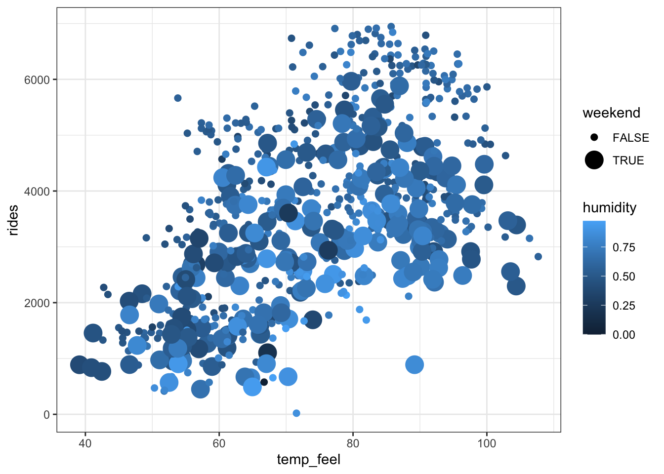


new_model_4 <- lm(rides ~ temp_feel + humidity + weekend, bikes)
summary(new_model_4)
## 
## Call:
## lm(formula = rides ~ temp_feel + humidity + weekend, data = bikes)
## 
## Residuals:
##     Min      1Q  Median      3Q     Max 
## -4052.0  -945.5   -34.0   848.0  2889.7 
## 
## Coefficients:
##              Estimate Std. Error t value Pr(>|t|)    
## (Intercept)   668.602    292.181   2.288   0.0224 *  
## temp_feel      59.368      3.119  19.033  < 2e-16 ***
## humidity    -1906.434    320.983  -5.939 4.43e-09 ***
## weekendTRUE  -869.058    100.058  -8.686  < 2e-16 ***
## ---
## Signif. codes:  0 '***' 0.001 '**' 0.01 '*' 0.05 '.' 0.1 ' ' 1
## 
## Residual standard error: 1223 on 727 degrees of freedom
## Multiple R-squared:  0.3882, Adjusted R-squared:  0.3856 
## F-statistic: 153.7 on 3 and 727 DF,  p-value: < 2.2e-16

On average, there are 669 riders on weekdays that feel like 0 degrees and have no humidity.
On days with the same humidity levels and time of the week, a 1 degree increase in temperature is associated with a 59 ride increase in average ridership.
On days with the same temperature and time of the week, a 0.1 point increase in humidity levels (i.e. a 1 percentage point increase in humidity) is associated with a 190.6 ride decrease in average ridership.
On days with the same temperature and humidity, the average ridership is 869 rides lower on weekends compared to weekdays.