14 Logistic wrap-up + project time

Announcements etc

SETTLING IN

Find the qmd here: “14-logistic-wrapup-project-notes.qmd”.

WRAPPING UP

Upcoming due dates:
- Today = PP 5
- Monday = Project group preference form
  This must be in on time so that I can have proposed groups in place on Tuesday!
- Tuesday = CP 12
Next Thursday (10/30): Quiz 2
- This will focus on the Multiple Linear Regression and Logistic Regression units, but is naturally cumulative.
- There’s a quiz review with Ryan on Sunday, 2-330.

Warm-up

Fake news is…a problem. Using data obtained from https://www.kaggle.com/mdepak/fakenewsnet, and cleaned using code provided at https://www.kaggle.com/kumudchauhan/fake-news-analysis-and-classification, we’ll try to predict if an article is fake news based on various features. NOTE: These data are from real articles posted online.

# Load packages and data
library(tidyverse)
fake_news <- read_csv("https://ajohns24.github.io/data/fake_news.csv") %>% 
  mutate(title_has_excl = title_excl > 0,
         is_fake = (type == "fake")) %>% 
  select(is_fake, title_has_excl, negative)

EXAMPLE 1: Intuition

We’ll explore the relationship of whether or not an article is_fake (TRUE or FALSE) with title_has_excl (whether the title has an exclamation point) and negative (the percent of words that have negative sentiment):

head(fake_news)

The model formula for this relationship is:

log(odds the article is fake) = \(\beta_0\) + \(\beta_1\) negative + \(\beta_2\) title_has_exclTRUE

Intuitively:

Do you think \(\beta_1\), the negative coefficient, will be positive or negative?
Do you think \(\beta_2\), the title_has_exclTRUE coefficient, will be positive or negative?

PAUSE: Build some plots and models of the relationships of interest

# Plot relationship of is_fake with title_has_excl
fake_news %>% 
  ggplot(aes(x = title_has_excl, fill = is_fake)) + 
  geom_bar(position = "fill")

# Plot relationship of is_fake with negative sentiment
fake_news %>% 
  mutate(negative_brackets = cut(negative, 15)) %>% 
  group_by(negative_brackets) %>% 
  summarize(fake_rate = mean(is_fake)) %>% 
  ggplot(aes(x = negative_brackets, y = fake_rate)) + 
  geom_point() + 
  theme(axis.text.x = element_text(angle = 60, vjust = 1, hjust=1))

# Model the relationship of is_fake with negative sentiment & title_has_excl
news_model <- glm(is_fake ~ title_has_excl + negative, fake_news, family = "binomial")
coef(summary(news_model))

# Plot the model on the probability scale
fake_news %>% 
  ggplot(aes(y = as.numeric(is_fake), x = negative, color = title_has_excl)) + 
  geom_smooth(method = "glm", se = FALSE, method.args = list(family = "binomial")) +
  labs(y = "probability of being fake") + 
  lims(y = c(0,1))

EXAMPLE 2: Interpret the coefficients of the estimated logistic regression model

log(odds the article is fake) = -1.8791 + 2.5265 title_has_exclTRUE + 0.3829 negative

# Exponentiated coefficients
exp(-1.8791)
exp(2.5265)
exp(0.3829)

Intercept:

title_has_exclTRUE coefficient:

negative coefficient (on your own):

EXAMPLE 3: How good is the model at distinguishing between real and fake news?

We can use our model to calculate the probability that an article is fake based on its negative sentiment score and whether or not its title includes an exclamation mark. Below are the probability calculations for the articles in our sample, split up by those that were & weren’t actually fake. Discuss.

fake_news %>% 
  mutate(.fitted = predict(news_model, newdata = ., type = "response")) %>% 
  ggplot(aes(x = is_fake, y = .fitted)) +
  geom_boxplot()

EXAMPLE 4: Evaluating the model (on your own)

Let’s explore using a probability threshold of 0.5 to make a binary prediction of an article’s status:

If the article’s probability of being fake is greater than or equal to 50%, we’ll predict that it’s fake.
Otherwise, we’ll predict that it’s real.

We can visualize this threshold on our predicted probability boxplots:

fake_news %>% 
  mutate(.fitted = predict(news_model, newdata = ., type = "response")) %>% 
  ggplot(aes(x = is_fake, y = .fitted)) +
  geom_boxplot() + 
  geom_hline(yintercept = 0.5, color = "red")

The resulting confusion matrix is below:

# Rows = actual / observed to be fake (FALSE or TRUE)
# Columns = predicted to be fake (FALSE or TRUE)
library(janitor)
threshold <- 0.5
fake_news %>% 
  mutate(.fitted = predict(news_model, newdata = ., type = "response")) %>% 
  mutate(predictFake = .fitted >= threshold) %>% 
  tabyl(is_fake, predictFake) %>%
  adorn_totals(c("row", "col"))

# Calculate the overall accuracy

# Calculate the sensitivity (true positive rate)

# Calculate the specificity (true negative rate)

QUESTION

In general, sensitivity & specificity are inversely related – increasing one leads to a decrease in the other. In this context, would you rather have high sensitivity or high specificity? Why?

EXAMPLE 5: Calculations (on your own)

Suppose you come across a news article that has an exclamation point in the title, and 4% of its words have a negative sentiment. Calculate the probability that this article is fake. You should make this calculation by hand, but can check it using predict():

predict(news_model, newdata = data.frame(title_has_excl = TRUE, negative = 4), type = "response")

EXAMPLE 6: Interaction (on your own)

data(penguins)
penguins_sub <- penguins %>% 
  filter(species %in% c("Adelie", "Gentoo"))

penguins_sub %>% 
  ggplot(aes(y = body_mass, x = flipper_len, color = species)) + 
  geom_smooth(method = "lm", se = FALSE)

In their relationship with body_mass, flipper_len and species interact. What does that mean?
The model formula can be expressed as:

E[body_mass | flipper_len, species] = \(\beta_0\) + \(\beta_1\) flipper_len + \(\beta_2\) speciesGentoo + \(\beta_3\) flipper_len * speciesGentoo

Indicate whether the coefficients below are positive or negative and what your reasoning is:
- \(\beta_1\)
- \(\beta_2\)
- \(\beta_3\)

EXAMPLE 7: More interaction (on your own)

summary(lm(body_mass ~ flipper_len*species, penguins_sub))

Write out separate sub-model formulas of body_mass vs flipper_len for Adelies and Gentoos.
Interpret the flipper_len and flipper_len:speciesGentoo coefficients.
Predict the body mass of a Gentoo penguin with 220mm long flippers.

Project intro

Project info & description
Project group preference form
- You cannot fill this out until after you’ve reviewed the data options!
- Due Monday by 11:59pm. Late forms will not be accepted for credit. I need this info in order to form suggested groups for Tuesday’s class.

Choose your own adventure

Finish the above examples. Let me know if you want to sit and work on them together!!
Finish PP 5 (due today)
Review the data options for the project & fill out the Project group preference form.
Start reviewing for Quiz 2 / putting together your note card.

Solutions

# Load packages and data
library(tidyverse)
fake_news <- read_csv("https://ajohns24.github.io/data/fake_news.csv") %>% 
  mutate(title_has_excl = title_excl > 0,
         is_fake = (type == "fake")) %>% 
  select(is_fake, title_has_excl, negative)

EXAMPLE 1: Intuition

Answers will vary!

head(fake_news)
## # A tibble: 6 × 3
##   is_fake title_has_excl negative
##   <lgl>   <lgl>             <dbl>
## 1 TRUE    FALSE              8.47
## 2 FALSE   FALSE              4.74
## 3 TRUE    TRUE               3.33
## 4 FALSE   FALSE              6.09
## 5 TRUE    FALSE              2.66
## 6 FALSE   FALSE              3.02

# Plot relationship of is_fake with title_has_excl
fake_news %>% 
  ggplot(aes(x = title_has_excl, fill = is_fake)) + 
  geom_bar(position = "fill")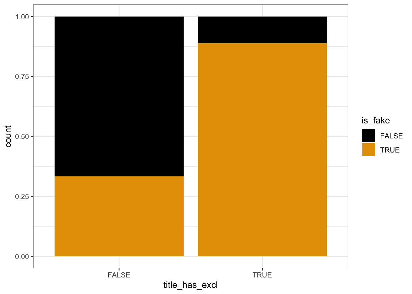


# Plot relationship of is_fake with negative sentiment
fake_news %>% 
  mutate(negative_brackets = cut(negative, 15)) %>% 
  group_by(negative_brackets) %>% 
  summarize(fake_rate = mean(is_fake)) %>% 
  ggplot(aes(x = negative_brackets, y = fake_rate)) + 
  geom_point() + 
  theme(axis.text.x = element_text(angle = 60, vjust = 1, hjust=1))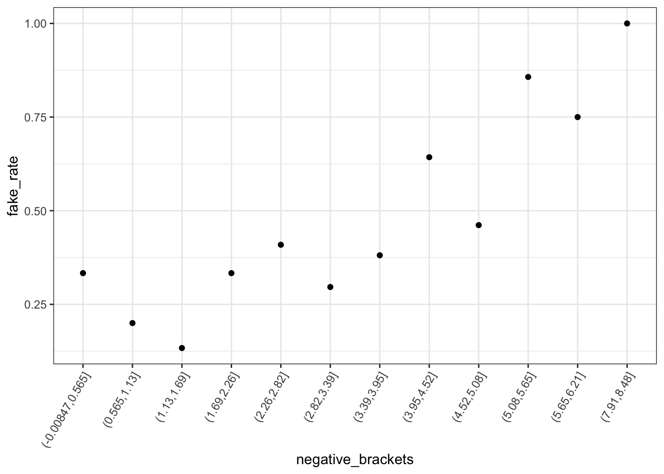


# Model the relationship of is_fake with negative sentiment & title_has_excl
news_model <- glm(is_fake ~ title_has_excl + negative, fake_news, family = "binomial")
coef(summary(news_model))
##                      Estimate Std. Error   z value     Pr(>|z|)
## (Intercept)        -1.8791361  0.5017141 -3.745432 0.0001800836
## title_has_exclTRUE  2.5264918  0.7858810  3.214853 0.0013051133
## negative            0.3828887  0.1464251  2.614912 0.0089250487

EXAMPLE 2: Interpret the coefficients of the estimated logistic regression model

# Exponentiate the coefficients
exp(-1.8791)
## [1] 0.1527275
exp(2.5265)
## [1] 12.50965
exp(0.3829)
## [1] 1.466531

Intercept: If an article does not have a “!” in the title and 0% of its words are negative, the odds that it’s fake are only 0.15. (The probability it’s fake is only 15% as high as the probability it’s real.)

title_has_exclTRUE coefficient: When controlling for an article’s negative sentiment (i.e. among articles that have the same negativity level), the odds of being fake are 12.5 times higher for articles that have an “!” in the title than for articles that don’t.

negative coefficient: When controlling for “!” use in the title (i.e. among both articles that do and don’t have an “!”), for every 1 percentage point increase in negative words, the odds of being fake increase by 47% (multiply by 1.47) on average.

EXAMPLE 3: How good is the model at distinguishing between real and fake news?

Mostly, the model assigns higher probabilities of being fake to articles that actually are fake than to articles that aren’t.

fake_news %>% 
  mutate(.fitted = predict(news_model, newdata = ., type = "response")) %>% 
  ggplot(aes(x = is_fake, y = .fitted)) +
  geom_boxplot()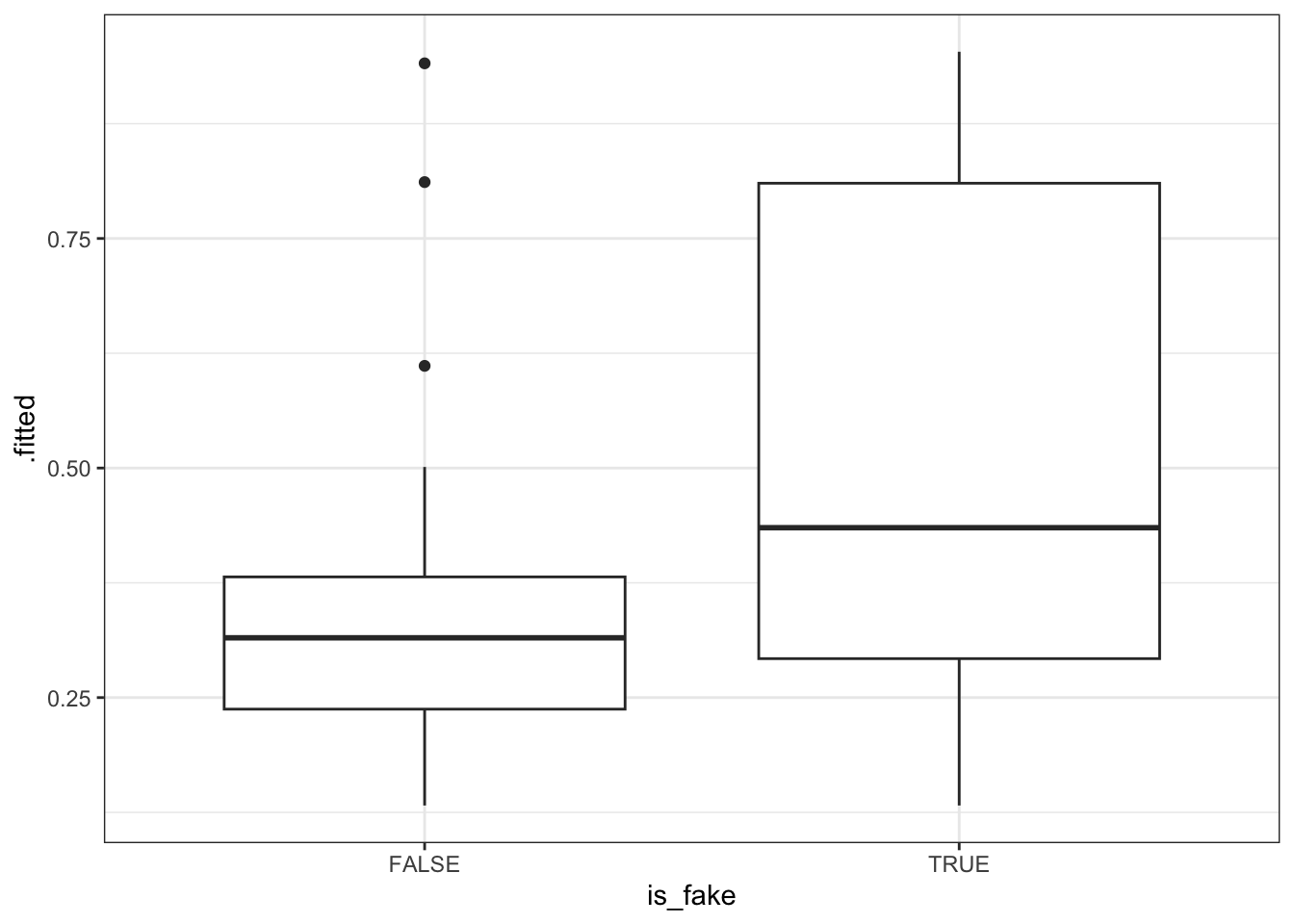

EXAMPLE 4: Evaluating the model (on your own)

# Rows = actual / observed to be fake (FALSE or TRUE)
# Columns = predicted to be fake (FALSE or TRUE)
library(janitor)
threshold <- 0.5
fake_news %>% 
  mutate(.fitted = predict(news_model, newdata = ., type = "response")) %>% 
  mutate(predictFake = .fitted >= threshold) %>% 
  tabyl(is_fake, predictFake) %>%
  adorn_totals(c("row", "col"))
##  is_fake FALSE TRUE Total
##    FALSE    86    4    90
##     TRUE    39   21    60
##    Total   125   25   150

# Calculate the overall accuracy
(86 + 21) / 150
## [1] 0.7133333

# Calculate the sensitivity (true positive rate)
21 / 60
## [1] 0.35

# Calculate the specificity (true negative rate)
86 / 90
## [1] 0.9555556

Whether sensitivity or specificity is better is subjective:

higher sensitivity: our model would be better at detecting when an article is fake, but at the cost of us mistaking real news for fake news.
higher specificity: our model would be better at detecting when an article is real, but at the cost of us more often mistaking fake news for real news.

EXAMPLE 5: Calculations (on your own)

# by hand
log_odds <- -1.8791 + 0.3829*4 + 2.5265*1
odds <- exp(log_odds)
prob <- odds / (odds + 1)
prob
## [1] 0.8983478


# Check
predict(news_model, newdata = data.frame(title_has_excl = TRUE, negative = 4), type = "response")
##         1 
## 0.8983396

EXAMPLE 6: Interaction (on your own)

data(penguins)
penguins_sub <- penguins %>% 
  filter(species %in% c("Adelie", "Gentoo"))

penguins_sub %>% 
  ggplot(aes(y = body_mass, x = flipper_len, color = species)) + 
  geom_smooth(method = "lm", se = FALSE)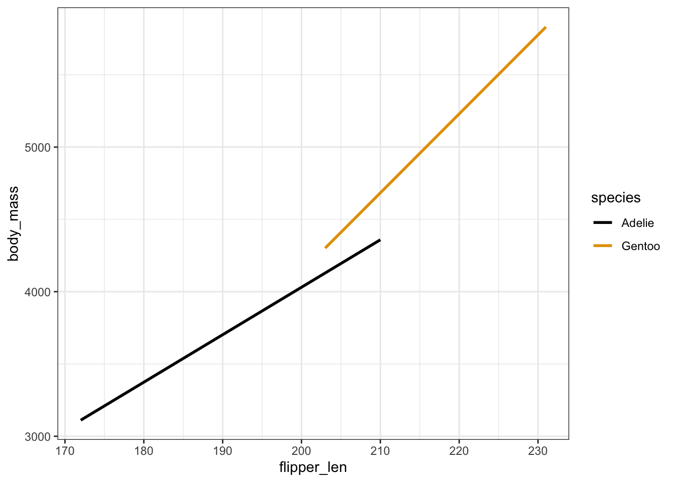

The relationship between body_mass and flipper_len varies by / is different for the 2 species.
.
- \(\beta_1 > 0\): This is the slope of the Adelie line. Among Adelies, the relationship between body mass and flipper length is positive.
- \(\beta_2 < 0\): This is the difference in the intercept of the Gentoo line relative to the Adelie line. The “baseline” body mass at a flipper length of 0 is lower among Gentoo than Adelie.
- \(\beta_3 > 0\): This is the difference in the slope of the Gentoo line relative to the Adelie line. The increase in body mass with flipper length is higher among Gentoo than Adelie.

EXAMPLE 7: More interaction (on your own)

summary(lm(body_mass ~ flipper_len*species, penguins_sub))
## 
## Call:
## lm(formula = body_mass ~ flipper_len * species, data = penguins_sub)
## 
## Residuals:
##     Min      1Q  Median      3Q     Max 
## -911.18 -265.28  -32.61  218.22 1144.81 
## 
## Coefficients:
##                            Estimate Std. Error t value Pr(>|t|)    
## (Intercept)               -2535.837    917.099  -2.765  0.00608 ** 
## flipper_len                  32.832      4.825   6.804 6.54e-11 ***
## speciesGentoo             -4251.444   1488.407  -2.856  0.00462 ** 
## flipper_len:speciesGentoo    21.791      7.238   3.011  0.00285 ** 
## ---
## Signif. codes:  0 '***' 0.001 '**' 0.01 '*' 0.05 '.' 0.1 ' ' 1
## 
## Residual standard error: 386.5 on 270 degrees of freedom
##   (2 observations deleted due to missingness)
## Multiple R-squared:  0.7886, Adjusted R-squared:  0.7863 
## F-statistic: 335.8 on 3 and 270 DF,  p-value: < 2.2e-16

.
- Adelie: E[body_mass|flipper_len] =-2535.837 + 32.832 flipper_lenProof: E[body_mass | flipper_len] = -2535.837 + 32.832 flipper_len - 4251.444*0 + 21.791*flipper_len*0
- Gentoo: E[body_mass|flipper_len] =-6787.281 + 54.623 flipper_lenProof: E[body_mass | flipper_len] = -2535.837 + 32.832 flipper_len - 4251.444*1 + 21.791*flipper_len*1 = (-2535.837 - 4251.444) + (32.832 + 21.791) flipper_len
For every 1cm increase in flipper length, the expected body mass increases by 32.8g for Adelies and by 21.8g more than that for Gentoos.

# Using the original model
-2535.837 + 32.832*220 - 4251.444*1 + 21.791*220*1
## [1] 5229.779

# Using the Gentoo sub-model
-6787.281 + 54.623*220
## [1] 5229.779