library(tidyverse)
titanic <- read_csv("https://mac-stat.github.io/data/titanic.csv") %>%
  mutate(Survived = as.factor(Survived)) %>%
  filter(!is.na(PClass))
head(titanic)
## # A tibble: 6 × 5
##   Name                                          PClass   Age Sex    Survived
##   <chr>                                         <chr>  <dbl> <chr>  <fct>
## 1 Allen, Miss Elisabeth Walton                  1st    29    female 1
## 2 Allison, Miss Helen Loraine                   1st     2    female 0
## 3 Allison, Mr Hudson Joshua Creighton           1st    30    male   0
## 4 Allison, Mrs Hudson JC (Bessie Waldo Daniels) 1st    25    female 0
## 5 Allison, Master Hudson Trevor                 1st     0.92 male   1
## 6 Anderson, Mr Harry 1st 47 male 112 Simple logistic regression
Announcements etc
SETTLING IN
- Today is a paper day! Put away laptops. You’ll need a basic calculator (possibly on your phone) that can calculate \(\log(x)\) and \(e^x = \text{exp}(x)\).
- After class, you can find the qmd here: “12-logistic-univariate-notes.qmd”.
WRAPPING UP
- Type up your notes in the qmd! This will be a good way to study.
- Today: PP 4 due
- Thursday: Fall break! There is nothing to do / think about for this class over break.
- After Fall break:
- Tuesday = CP 11 (You’re encouraged to do this Monday, not over break.)
- Thursday = PP 5
- Thursday, Oct 30 = Quiz 2
This will focus on the Multiple Linear Regression and Logistic Regression units, but is naturally cumulative.
Learning goals
- Distinguish between probabilities and odds, and convert one to the other
- Explain the differences between linear regression and logistic regression for modeling binary outcomes
- Explore simple logistic regression models
- visualize relationships
- build models in R
- interpret coefficients
- make predictions
- converting from log odds to odds to probability scales
Additional resources
References
Logistic Regression
Let \(Y\) be a binary categorical response variable:
\[Y = \begin{cases} 1 & \; \text{ if event happens} \\ 0 & \; \text{ if event doesn't happen} \\ \end{cases}\]
Further define
\[\begin{split} p &= \text{ probability event happens} \\ 1-p &= \text{ probability event doesn't happen} \\ \text{odds} & = \text{ odds event happens} = \frac{p}{1-p} \\ \end{split}\]
Then a logistic regression model of \(Y\) by \(x\) is \[\log(\text{odds}) = \beta_0 + \beta_1 X\]
We can transform this to get (curved) models of odds and probability:
\[\begin{split} \text{odds} & = e^{\beta_0 + \beta_1 X} \\ p & = \frac{\text{odds}}{\text{odds}+1} = \frac{e^{\beta_0 + \beta_1 X}}{e^{\beta_0 + \beta_1 X}+1} \\ \end{split}\]
Warm-up
We’ve been focusing on “Normal” linear regression models for quantitative response variables Y. But not all response variables are quantitative! We’ll now explore logistic regression models for binary categorical response variables Y. This dramatically expands the types of relationships we’re able to explore. Though the details of our models will change, the spirit and considerations are the same:
- we want to learn about Y from predictors X
- we want to build, interpret, and evaluate our models
- we need to be mindful of multicollinearity, overfitting, etc in this process
EXAMPLE 1: Normal or logistic?
For each scenario below, indicate whether “Normal” or logistic regression would be the appropriate modeling tool.
We want to model a person’s commute time (Y) by their distance to work (X).
We want to model a person’s commute time (Y) by whether or not they take public transit (X).
We want to model whether or not a person gets a speeding ticket (Y) based on their driving speed (X).
EXAMPLE 2: probability vs odds vs log(odds)
- There’s a 0.9 probability that your team wins its next game. Calculate the corresponding odds and log(odds) of this event. NOTE:
log()is the natural log function in RStudio.
- The log(odds) that your bus is late are -1.0986. Calculate the corresponding odds and probability of this event. NOTE: Use
exp().
EXAMPLE 3: Conditional odds
The Titanic was a British passenger ship that famously sank in 1912 after hitting an iceberg in the North Atlantic Ocean. Approximately 2200 passengers were on board, and it’s estimated that 1500 did not survive the crash. The titanic dataset has info on a sample of these passengers:
Let’s use it to explore the relationship of:
- Y =
Survived(1 = survived, 0 = did not survive) - X =
PClass(ticket class = 1st, 2nd, 3rd)
To this end, check out some tables of counts:
titanic %>%
  count(PClass, Survived)
## # A tibble: 6 × 3
##   PClass Survived     n
##   <chr>  <fct>    <int>
## 1 1st    0          129
## 2 1st    1          193
## 3 2nd    0          160
## 4 2nd    1          119
## 5 3rd    0          573
## 6 3rd    1          138

library(janitor)
titanic %>%
  tabyl(PClass, Survived) %>%
  adorn_totals(c("row", "col"))
##  PClass   0   1 Total
##     1st 129 193   322
##     2nd 160 119   279
##     3rd 573 138   711
##   Total 862 450  1312
And a plot of Y alone, and 2 plots of Y with X.
titanic %>%
  ggplot(aes(x = Survived)) +
  geom_bar() +
theme_bw() 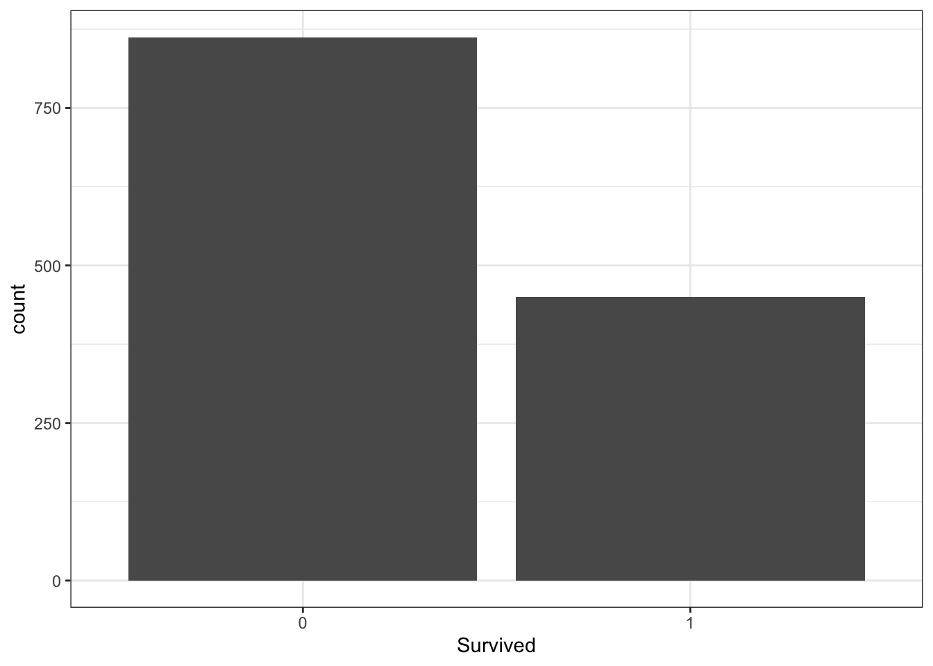
titanic %>%
  ggplot(aes(x = PClass, fill = Survived)) +
  geom_bar() +
  theme_bw()  +
  theme(legend.position = "bottom")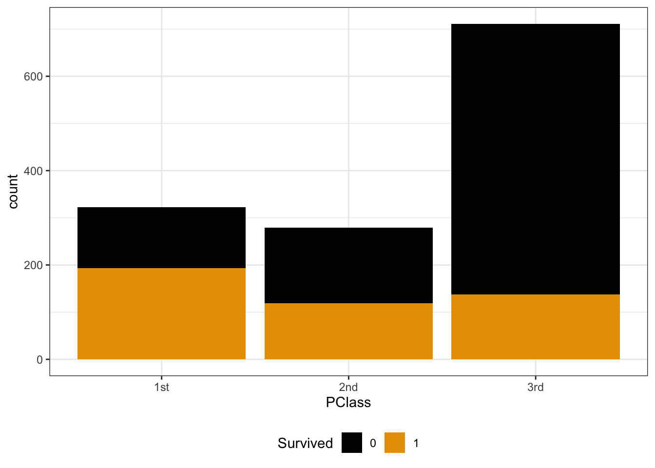
titanic %>%
  ggplot(aes(x = PClass, fill = Survived)) +
  geom_bar(position = "fill") +
  theme_bw() +
  theme(legend.position = "bottom")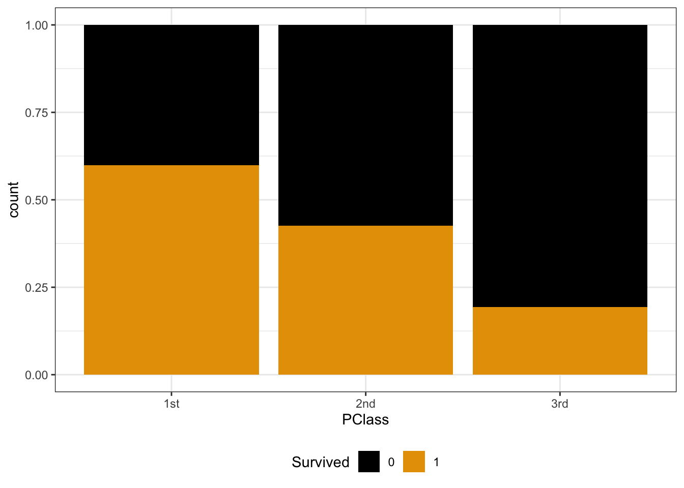
Calculate the overall odds that a passenger survived. (Which plot provides insight here?)
Y and X are both categorical. To visualize their relationship, we can make bar plots of X, split up by category of Y. Use plots 2 & 3 to describe the relationship of survival with ticket class. (What’s the difference between these plots, and which plot makes it easier to answer this question?!)
How does Y depend upon X? Calculate the conditional odds that a 1st class passenger survived, i.e. the odds of survival conditioned on the passenger being 1st class: Odds(survive | 1st class)
Calculate the conditional odds that a 3rd class passenger survived: Odds(survive | 3rd class)
EXAMPLE 4: Odds ratios
Models help us compare the behavior of Y for different possible X values. In logistic regression, these comparisons are often measured by odds ratios, a ratio of odds (unsurprisingly) that compares the odds of one group to another.
Calculate & interpret the odds ratio of surviving the Titanic, comparing those in the 1st class to those in the 3rd class.
Calculate & interpret the odds ratio of surviving the Titanic, comparing those in the 3rd class to those in the 1st class.
Odds ratios
Let “odds for group A” be the conditional odds of an event for some group A. Let “odds for group B” be the conditional odds of an event for some group B. Then the odds ratio (OR) of the event, comparing group A to group B is
OR = (odds for group A) / (odds for group B)
Then OR >= 0 where:
If OR > 1, then the odds of the event are higher for group A than group B. Examples:
- OR = 2: The odds of the event are 2 times higher (100% higher) for group A than group B.
- OR = 1.5: The odds of the event are one and a half times higher (50% higher) for group A than group B.
If OR = 1, then the odds of the event are the same for groups A and B.
If OR < 1, then the odds of the event are lower for group A than group B. Examples:
- OR = 0.5: The odds of the event are half as high (50% as high) for group A than group B.
- OR = 0.2:
- The odds of the event for group A are 0.2 times (20% as high as) the odds for group B.
- The odds of the event are 80% lower for group A than group B.
Exercises
Directions
There’s a lot of new and specialized syntax today. Peak at but not get distracted by the syntax – stay focused on the bigger picture concepts.
The story
The climbers data is sub-sample of the Himalayan Database distributed through the R for Data Science TidyTuesday project. This dataset includes information on the results and conditions for various Himalayan climbing expeditions. Each row corresponds to a single member of a climbing expedition team:
# Load packages and data
library(tidyverse)
climbers <- read_csv("https://mac-stat.github.io/data/climbers_sub.csv") %>%
  select(peak_name, success, age, oxygen_used, height_metres)

# Check out the first 6 rows
head(climbers)
## # A tibble: 6 × 5
##   peak_name  success   age oxygen_used height_metres
##   <chr>      <lgl>   <dbl> <lgl>               <dbl>
## 1 Ama Dablam TRUE       28 FALSE                6814
## 2 Ama Dablam TRUE       27 FALSE                6814
## 3 Ama Dablam TRUE       35 FALSE                6814
## 4 Ama Dablam TRUE       37 FALSE                6814
## 5 Ama Dablam TRUE       43 FALSE                6814
## 6 Ama Dablam FALSE      38 FALSE                6814
Our goal will be to model whether or not a climber has success (Y) by their age (in years) or oxygen_used (TRUE or FALSE). Since success is a binary categorical variable, i.e. a climber is either successful or they’re not, we’ll utilize logistic regression.
Exercise 1: Getting to know Y
Our response variable Y, success, is binary (hence categorical). Thus we can explore Y alone using a bar plot and table of counts. Discuss what you learn here.
climbers %>%
  count(success)
## # A tibble: 2 × 2
##   success     n
##   <lgl>   <int>
## 1 FALSE    1269
## 2 TRUE      807
climbers %>%
  ggplot(aes(x = success)) +
  geom_bar()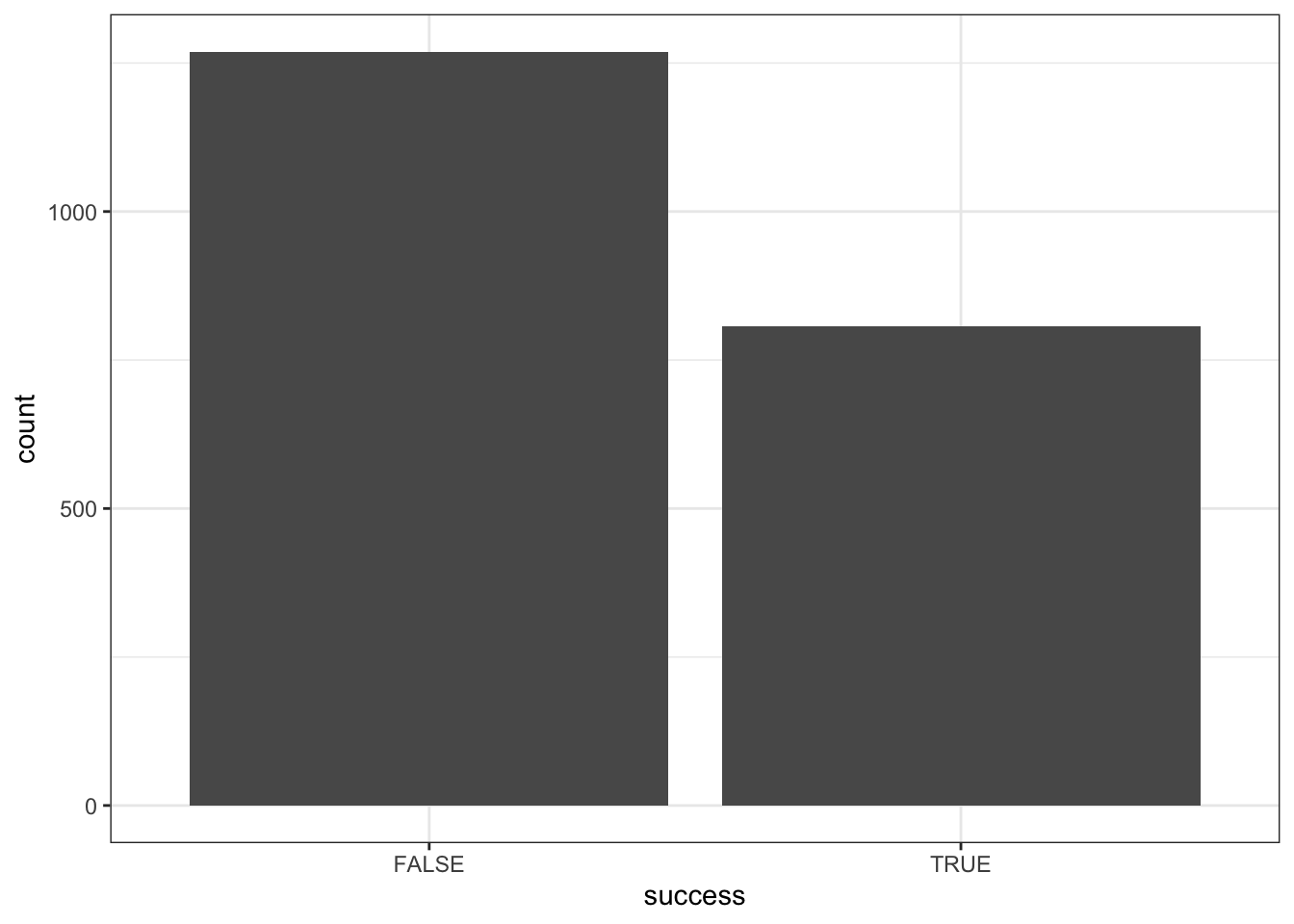
Exercise 2: Visualizing success vs age
Let’s now explore the relationship of success with age. Since success (Y) is categorical and age (X) is quantitative, it can be tempting to draw something like a side-by-side boxplot:
climbers %>%
  ggplot(aes(y = age, x = success)) +
  geom_boxplot()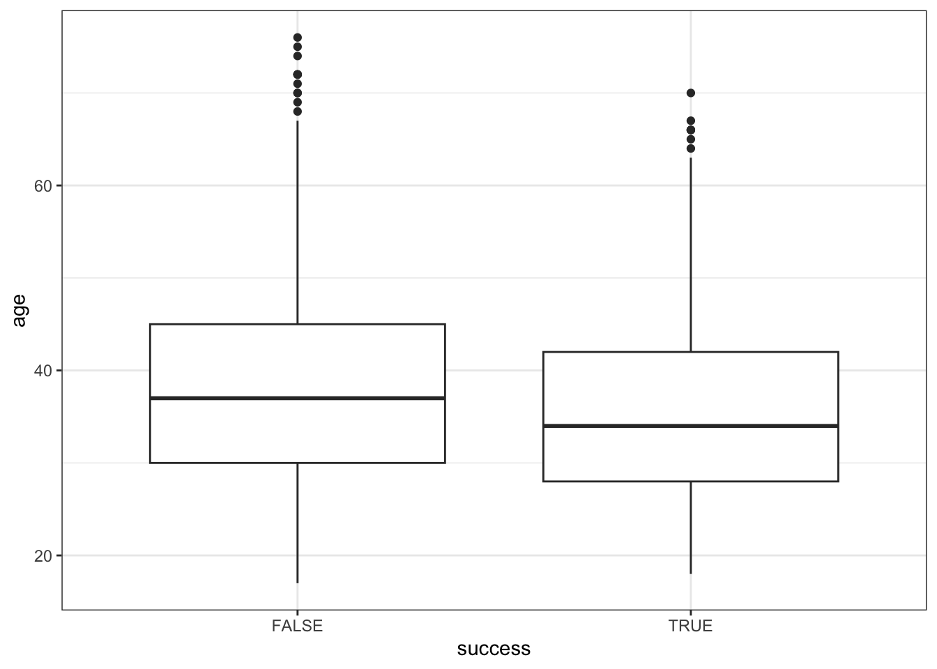
BUT this only gives us insight into the dependence of age on success, not success on age (it reverses the roles of Y and X). Instead, we want to calculate the observed success rate (probability of success) at each age, or in each age bracket.
Part a
Below is a summary of successes and failures at different ages. Calculate the observed success rate (probability of success) for…
18 year olds: ____ / (3 + 4) =
17-19 year olds: ___ / (1 + 4 + 3 + 4 + 8) =
climbers %>%
  count(age, success) %>%
  head(5)
## # A tibble: 5 × 3
##     age success     n
##   <dbl> <lgl>   <int>
## 1    17 FALSE       1
## 2    18 FALSE       4
## 3    18 TRUE        3
## 4    19 FALSE       4
## 5    19 TRUE        8
Part b
We can calculate these success rates using group_by() and summarize(). Check that these are consistent with your answers to Part a:
# Calculate success rate by age
climbers %>%
  group_by(age) %>%
  summarize(success_rate = mean(success)) %>%
  head(3)
## # A tibble: 3 × 2
##     age success_rate
##   <dbl>        <dbl>
## 1    17        0
## 2    18        0.429
## 3    19        0.667

# Split climbers into larger, more stable age brackets
# (This is good when we don't have many observations at each x!)
# Calculate success rate by age bracket
climbers %>%
  mutate(age_bracket = cut(age, breaks = 20)) %>%
  group_by(age_bracket) %>%
  summarize(success_rate = mean(success)) %>%
  head(3)
## # A tibble: 3 × 2
##   age_bracket success_rate
##   <fct>              <dbl>
## 1 (16.9,19.9]        0.55
## 2 (19.9,22.9]        0.584
## 3 (22.9,25.9]        0.432
Now, plot the success rates by age and age bracket below. Summarize what you learn about the relationship (note that we weren’t able to observe this information from the boxplots!).
climbers %>%
  group_by(age) %>%
  summarize(success_rate = mean(success)) %>%
  ggplot(aes(x = age, y = success_rate)) +
  geom_point()
climbers %>%
  mutate(age_bracket = cut(age, breaks = 20)) %>%
  group_by(age_bracket) %>%
  summarize(success_rate = mean(success)) %>%
  ggplot(aes(x = age_bracket, y = success_rate)) +
  geom_point() +
  theme(axis.text.x = element_text(angle = 90, vjust = 0.5, hjust=1))
Exercise 3: Logistic regression in R
To model the relationship between success and age, we can construct the logistic regression model using the code below. Point out the 2 new things about this code.
climbing_model_1 <- glm(success ~ age, data = climbers, family = "binomial")
coef(summary(climbing_model_1))
##                Estimate  Std. Error   z value     Pr(>|z|)
## (Intercept)  0.42568563 0.169177382  2.516209 1.186249e-02
## age         -0.02397199 0.004489504 -5.339564 9.317048e-08
Exercise 4: Writing out & plotting the model
The estimated model formula is stated below on the log(odds), odds, and probability scales.
log(odds of success) = 0.42569 - 0.02397age
odds of success = \(e^{0.42569 - 0.02397\text{age}}\)
probability of success = \(e^{0.42569 - 0.02397\text{age}}\) / (\(e^{0.42569 - 0.02397\text{age}}\) + 1)
Part a
Convince yourselves that you know where the above formulas come from!
Part b
Our one model, expressed on different scales, is plotted below. As with the plot of our data on success rates in Exercise 3, these indicate that success rate decreases with age. (This is true on every scale, of course.) Compare the shapes of the models on these different scales.
- Which model is linear?
- Which model is S-shaped?
- Which model is restricted between 0 and 1 on the y-axis?
- Which model is curved and restricted to be above 0 (but not necessarily below 1) on the y-axis?
# Incorporate predictions on the probability, odds, & log-odds scales
climbers_predictions <- climbers %>%
  mutate(probability = climbing_model_1$fitted.values) %>%
  mutate(odds = probability / (1-probability)) %>%
  mutate(log_odds = log(odds))

# Plot the model on the log-odds scale
ggplot(climbers_predictions, aes(x = age, y = log_odds)) +
geom_smooth(se = FALSE) 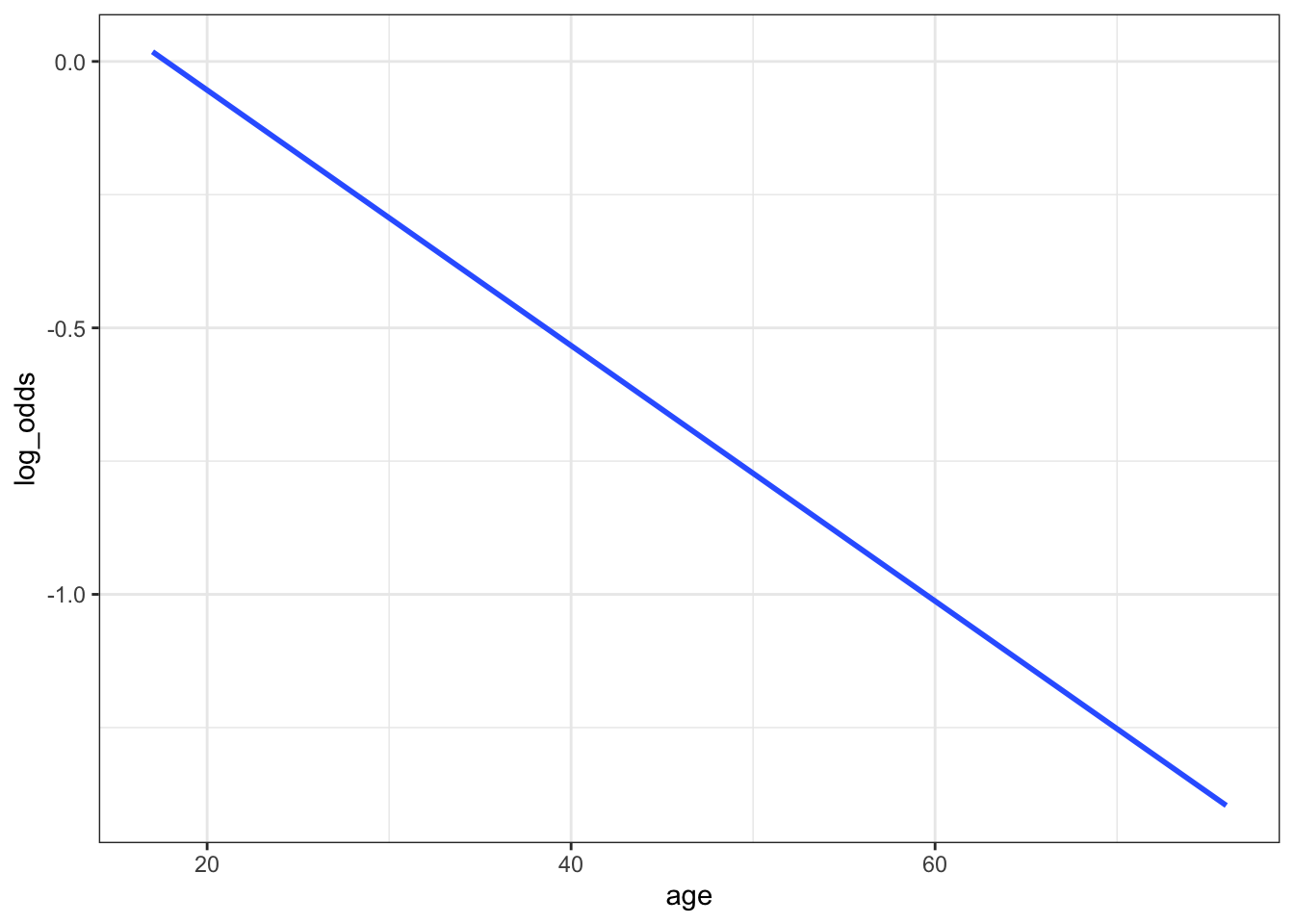
# Plot the model on the odds scale
ggplot(climbers_predictions, aes(x = age, y = odds)) +
geom_smooth(se = FALSE) 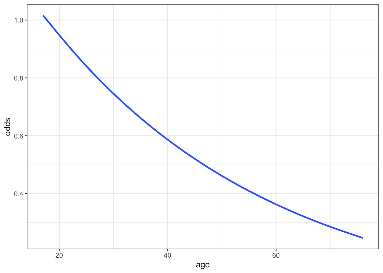
# Plot the model on the probability scale
ggplot(climbers_predictions, aes(x = age, y = probability)) +
geom_smooth(se = FALSE) 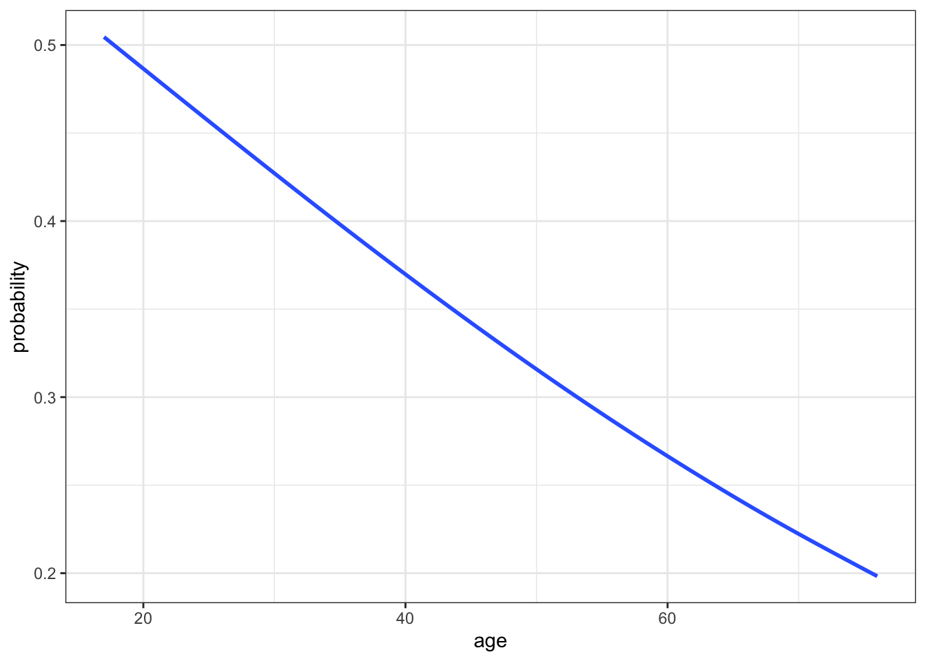
#...and zoom out to see broader (and impossible) age range
ggplot(climbers_predictions, aes(x = age, y = as.numeric(success))) +
  geom_smooth(method = "glm", method.args = list(family = "binomial"), se = FALSE, fullrange = TRUE) +
  labs(y = "probability") +
  lims(x = c(-200,200))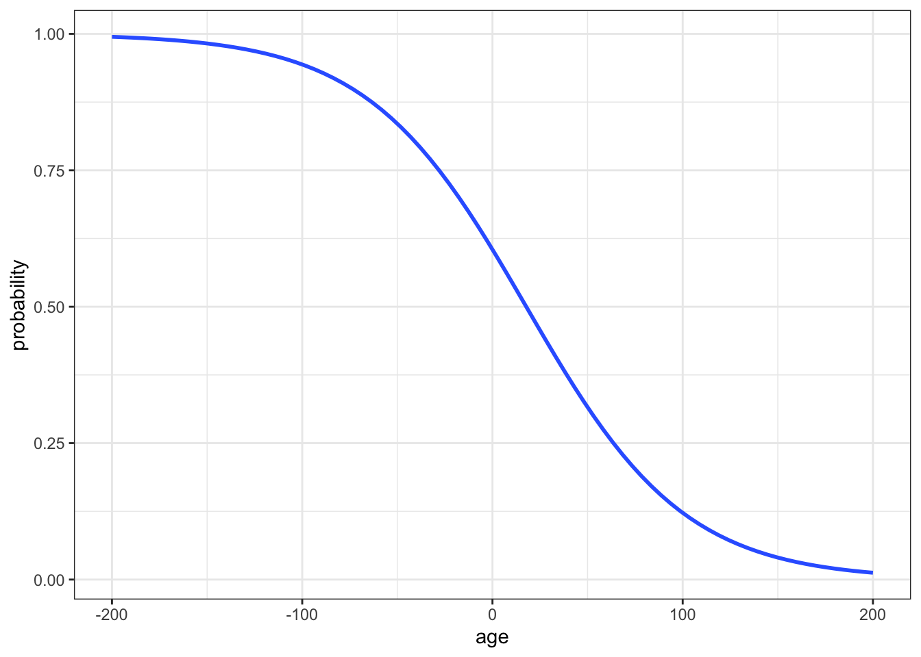
Exercise 5: Predictions
Let’s use the model formulas from the above exercise to make predictions. Consider a 20-year-old climber.
Part a
Calculate the log(odds) that this climber will succeed. HINT: use the log(odds) model.
Part b
Calculate the odds that this climber will succeed. HINT: Either transform the log(odds) prediction or use the odds model.
Part c
Calculate the probability that this climber will succeed. HINT: Either transform the odds prediction or use the probability model.
Part d
Check your calculations 2 ways:
- Are they consistent with the model visualizations above?
- Do they match the results of the
predict()function?
# Check the log-odds prediction
predict(climbing_model_1, newdata = data.frame(age = 20))
##           1
## -0.05375421

# Check the odds prediction
exp(predict(climbing_model_1, newdata = data.frame(age = 20)))
##        1
## 0.947665

# Check the probability prediction
predict(climbing_model_1, newdata = data.frame(age = 20), type = "response")
##         1
## 0.4865647
Exercise 6: Interpreting the intercept
In using the logistic regression model, it’s important to interpret the coefficients. Let’s learn how to do that, starting with the intercept of our model: log(odds of success) = 0.42569 - 0.02397age. Since the model on the log(odds) scale is just a line, we can interpret the intercept as usual:
Among 0 year old climbers (lol), the log(odds of success) is 0.42569.
But who cares?! It’s tough to interpret log(odds). Translate that statement to the odds scale:
Among 0 year old climbers (lol), the odds of success are…
Exercise 7: Interpreting the age coefficient
Since the model on the log(odds) scale is just a line, we can also interpret the age coefficient as the slope of that line:
A 1-year increase in age is associated with a decrease of 0.02397 in the log(odds of success), on average.
Again, since that’s hard to understand, we can convert the age coefficient to the odds scale: \(e^{-0.02397} = 0.976313\). BUT since the odds model is NOT linear, we can’t interpret this as a slope. So what does it mean?
Part a
Below are the odds of success among various ages:
exp(predict(climbing_model_1, newdata = data.frame(age = 23)))
##         1
## 0.8819057
exp(predict(climbing_model_1, newdata = data.frame(age = 22)))
##         1
## 0.9033021
exp(predict(climbing_model_1, newdata = data.frame(age = 21)))
##         1
## 0.9252177
exp(predict(climbing_model_1, newdata = data.frame(age = 20)))
##        1
## 0.947665
Calculate and interpret the odds ratio of success, comparing 23-year-olds to 22-year-olds. (Do not use rounded numbers in this calculation or those below!)
Part b
Calculate and interpret the odds ratio of success, comparing 22-year-olds to 21-year-olds.
Part c
Calculate and interpret the odds ratio of success, comparing 21-year-olds to 20-year-olds.
Part d
Summarize the punchline here.
On the log(odds) scale, the
agecoefficient is 0.02397:
On average, for every 1-year increase in age, log(odds of success) decrease by 0.02397.On the odds scale, the
agecoefficient is \(e^{-0.02397} = 0.976313\):
On average, for every 1-year increase in age, odds of success are ???% as high.That is, they decrease by ???%
Exercise 8: Another climbing model
Next, let’s explore the relationship of success (Y) with oxygen_used (X). Since both variables are categorical, we can fill in a bar plot of X with the categories of Y:
# Plot the relationship
climbers %>%
  ggplot(aes(x = oxygen_used, fill = success)) +
  geom_bar(position = "fill")
# Model the relationship
climbing_model_2 <- glm(success ~ oxygen_used, data = climbers, family = "binomial")
coef(summary(climbing_model_2))
##                  Estimate Std. Error   z value      Pr(>|z|)
## (Intercept)     -1.327993  0.0639834 -20.75528  1.098514e-95
## oxygen_usedTRUE  2.903864  0.1257404  23.09412 5.304291e-118
Thus the estimated model formula is:
log(odds of success) = -1.327993 + 2.903864 oxygen_usedTRUE
Part a
Describe what you learn about the relationship from the plot alone.
Part b
Calculate:
- the odds of success for a climber that doesn’t use oxygen
- the probability of success for a climber that doesn’t use oxygen
Part c
Calculate:
- the odds of success for a climber that uses oxygen
- the probability of success for a climber that uses oxygen
Part d
Check that your probability and odds calculations match those below:
exp(predict(climbing_model_2, newdata = data.frame(oxygen_used = FALSE)))
##         1
## 0.2650086
predict(climbing_model_2, newdata = data.frame(oxygen_used = FALSE), type = "response")
##         1
## 0.2094915
exp(predict(climbing_model_2, newdata = data.frame(oxygen_used = TRUE)))
##        1
## 4.834951
predict(climbing_model_2, newdata = data.frame(oxygen_used = TRUE), type = "response")
##        1
## 0.828619
Part e
Calculate and interpret the odds ratio of success, comparing climbers that do use oxygen to those that don’t. NOTE: Your calculation should be above 1!!
Exercise 9: Interpreting coefficients
Let’s interpret the coefficients of our logistic regression model:
log(odds of success) = -1.327993 + 2.903864 oxygen_usedTRUE
On the log(odds) scale:
- The log(odds of success) for climbers that don’t use oxygen is -1.327993.
- The log(odds of success) is 2.903864 higher for climbers that use oxygen than for those that don’t.
Yuk. Convert those coefficients to the odds scale:
exp(-1.327993)
exp(2.903864)
Part a
How can we interpret the intercept on the odds scale, 0.265? Where have you observed this number before?!
Part b
How can we interpret the oxygen_usedTRUE coefficient on the odds scale, 18.24? Where have you observed this number before?!
Exercise 10: Connecting tables to logistic regression
For the simple logistic regression model with 1 predictor, which is categorical, the model coefficients can be calculated from the table of counts! Here rows represent whether oxygen was used and columns represent whether the climber was successful:
# Rows correspond to oxygen_used
# Columns correspond to success
climbers %>%
  tabyl(oxygen_used, success) %>%
  adorn_totals(c("row", "col"))
##  oxygen_used FALSE TRUE Total
##        FALSE  1166  309  1475
##         TRUE   103  498   601
##        Total  1269  807  2076
Part a
Use this table to calculate the odds of success for somebody that didn’t use oxygen. Where have you observed this number before?! HINT: Use the FALSE row.
Part b
Use this table to calculate the odds ratio of success, comparing climbers that do use oxygen to those that don’t. Where have you observed this number before?! HINT: You’ll first need to calculate the odds of success for people that use oxygen.
Exercise 11: Interpreting logistic regression coefficients
In general (not just for climbers), let’s summarize how to interpret logistic regression coefficients. Review the details below and convince yourself that these general properties are consistent with your work above. Let \(Y\) be a binary categorical response variable (eg: Y = 1 if the event of interest happens and is 0 otherwise). Then a logistic regression model of \(Y\) by \(Y\) is
\[\log(\text{odds}) = \beta_0 + \beta_1 X\]
- Coefficient interpretation for quantitative X
\[\begin{split} \beta_0 & = \text{ LOG(ODDS) when } X=0 \\ e^{\beta_0} & = \text{ ODDS when } X=0 \\ \beta_1 & = \text{ change in LOG(ODDS) per 1 unit increase in } X \\ e^{\beta_1} & = \text{ multiplicative change in ODDS per 1 unit increase in } X \text{ (ie. the odds ratio, comparing the odds for X + 1 vs X)} \\ \end{split}\] - Coefficient interpretation for categorical X
\[\begin{split} \beta_0 & = \text{ LOG(ODDS) at the reference category } \\ e^{\beta_0} & = \text{ ODDS at the reference category } \\ \beta_1 & = \text{ unit change in LOG(ODDS) relative to the reference} \\ e^{\beta_1} & = \text{ multiplicative change in ODDS relative to the reference } \text{ (ie. the odds ratio, comparing the odds for the given category vs the reference category)} \\ \end{split}\]
Exercise 12: R code
A lot of R code was used to produce the plots and other output above. The code is not the point. It’s more important to understand the logistic regression concepts, and the output of the code – you can always look up code. With that in mind, review the code to get a sense for the structure!
Exercise 13: VERY optional math challenge
Consider a simple logistic regression model:
\[\log(\text{odds}) = \beta_0 + \beta_1 X\]
Prove that \(e^{\beta_1}\) indicates the MULTIPLICATIVE change in ODDS for a 1-unit increase in X, i.e. that it’s equivalent to the odds ratio for “X+1” vs “X”.
Solutions
EXAMPLE 1: Normal or logistic?
- Normal. Y is quantitative.
- Normal. Y is quantitative.
- Logistic. Y is binary.
EXAMPLE 2: probability vs odds vs log(odds)
# a.
# odds
0.9 / (1 - 0.9)
# log(odds)
log(9)

# b.
# odds
exp(-1.0986)
# prob
0.333 / (0.333 + 1)
EXAMPLE 3: Conditional odds
library(tidyverse)
titanic <- read_csv("https://mac-stat.github.io/data/titanic.csv")
head(titanic)
## # A tibble: 6 × 5
##   Name                                          PClass   Age Sex    Survived
##   <chr>                                         <chr>  <dbl> <chr>     <dbl>
## 1 Allen, Miss Elisabeth Walton                  1st    29    female        1
## 2 Allison, Miss Helen Loraine                   1st     2    female        0
## 3 Allison, Mr Hudson Joshua Creighton           1st    30    male          0
## 4 Allison, Mrs Hudson JC (Bessie Waldo Daniels) 1st    25    female        0
## 5 Allison, Master Hudson Trevor                 1st     0.92 male          1
## 6 Anderson, Mr Harry                            1st    47    male          1

titanic %>%
  count(PClass, Survived)
## # A tibble: 7 × 3
##   PClass Survived     n
##   <chr>     <dbl> <int>
## 1 1st           0   129
## 2 1st           1   193
## 3 2nd           0   160
## 4 2nd           1   119
## 5 3rd           0   573
## 6 3rd           1   138
## 7 <NA>          0     1

library(janitor)
titanic %>%
  tabyl(PClass, Survived, show_na = FALSE) %>%
  adorn_totals(c("row", "col"))
##  PClass   0   1 Total
##     1st 129 193   322
##     2nd 160 119   279
##     3rd 573 138   711
##   Total 862 450  1312
.
# probability of survival
450 / 1312
# odds of survival
(450 / 1312) / (1 - (450 / 1312))
Survival was most likely for 1st class passengers and least likely for 3rd class passengers. NOTE: The first plot makes more clear that there were more 3rd class passengers, but the second plot makes it easier to compare survival rates among each class.
titanic %>%
  ggplot(aes(x = PClass, fill = factor(Survived))) +
  geom_bar()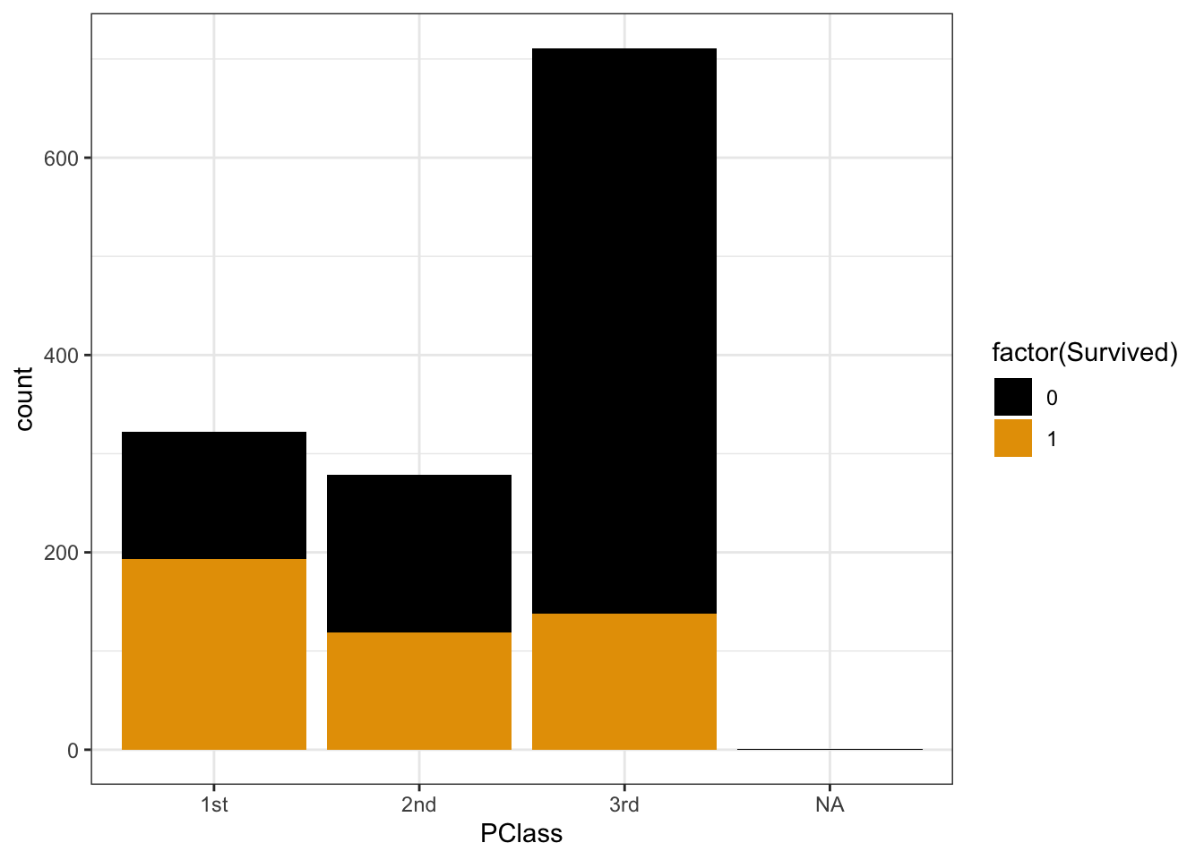
titanic %>%
  ggplot(aes(x = PClass, fill = factor(Survived))) +
  geom_bar(position = "fill")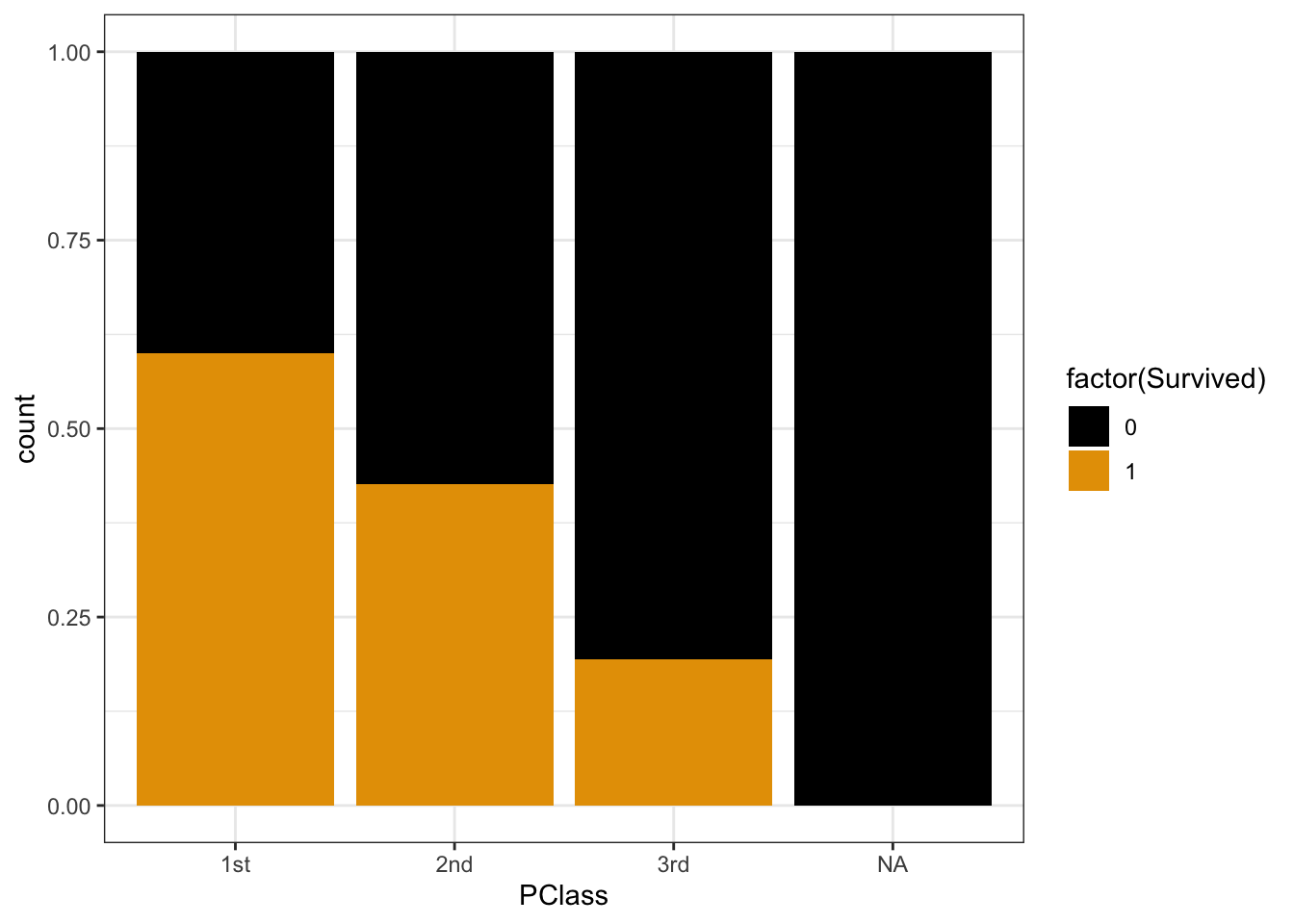
.
# probability of survival for 1st class
193 / 322
## [1] 0.5993789
# odds of survival for 1st class
(193 / 322) / (1 - (193 / 322))
## [1] 1.496124
.
# probability of survival for 3rd class
138 / 711
## [1] 0.1940928
# odds of survival for 3rd class
(138 / 711) / (1 - (138 / 711))
## [1] 0.2408377
EXAMPLE 4: Odds ratios
The odds of survival were more than 6 times higher for 1st class vs 3rd class:
# odds of survival for 1st class / odds of survival for 3rd class
1.50 / 0.24
The odds of survival for 3rd class passengers were only 16% as high as those for 1st class passengers (i.e. they were 84% lower):
# odds of survival for 3rd class / odds of survival for 1st class
0.24 / 1.50
# Load packages and data
library(tidyverse)
climbers <- read_csv("https://mac-stat.github.io/data/climbers_sub.csv") %>%
  select(peak_name, success, age, oxygen_used, height_metres)

# Check out the first 6 rows
head(climbers)
## # A tibble: 6 × 5
##   peak_name  success   age oxygen_used height_metres
##   <chr>      <lgl>   <dbl> <lgl>               <dbl>
## 1 Ama Dablam TRUE       28 FALSE                6814
## 2 Ama Dablam TRUE       27 FALSE                6814
## 3 Ama Dablam TRUE       35 FALSE                6814
## 4 Ama Dablam TRUE       37 FALSE                6814
## 5 Ama Dablam TRUE       43 FALSE                6814
## 6 Ama Dablam FALSE      38 FALSE                6814
Exercise 1: Getting to know Y
Roughly 40% of climbers succeed.
climbers %>%
  count(success)
## # A tibble: 2 × 2
##   success     n
##   <lgl>   <int>
## 1 FALSE    1269
## 2 TRUE      807
climbers %>%
  ggplot(aes(x = success)) +
  geom_bar()
Exercise 2: Visualizing success vs age
Part a
climbers %>%
  count(age, success) %>%
  head(5)
## # A tibble: 5 × 3
##     age success     n
##   <dbl> <lgl>   <int>
## 1    17 FALSE       1
## 2    18 FALSE       4
## 3    18 TRUE        3
## 4    19 FALSE       4
## 5    19 TRUE        8
18 year olds: 3 / (3 + 4) = 0.43
17-19 year olds: (3 + 8) / (1 + 4 + 3 + 4 + 8) = 0.55
Part b
Success rates start at nearly 60% for teenagers, then decrease with age – success rates approach 0 for climbers in their 70s.
# Calculate success rate by age
climbers %>%
  group_by(age) %>%
  summarize(success_rate = mean(success))
## # A tibble: 59 × 2
##      age success_rate
##    <dbl>        <dbl>
##  1    17        0
##  2    18        0.429
##  3    19        0.667
##  4    20        0.857
##  5    21        0.577
##  6    22        0.486
##  7    23        0.526
##  8    24        0.333
##  9    25        0.463
## 10    26        0.413
## # ℹ 49 more rows

# Split climbers into larger, more stable age brackets
# (This is good when we don't have many observations at each x!)
# Calculate success rate by age bracket
climbers %>%
  mutate(age_bracket = cut(age, breaks = 20)) %>%
  group_by(age_bracket)
## # A tibble: 2,076 × 6
## # Groups:   age_bracket [20]
##    peak_name  success   age oxygen_used height_metres age_bracket
##    <chr>      <lgl>   <dbl> <lgl>               <dbl> <fct>
##  1 Ama Dablam TRUE       28 FALSE                6814 (25.9,28.8]
##  2 Ama Dablam TRUE       27 FALSE                6814 (25.9,28.8]
##  3 Ama Dablam TRUE       35 FALSE                6814 (34.7,37.6]
##  4 Ama Dablam TRUE       37 FALSE                6814 (34.7,37.6]
##  5 Ama Dablam TRUE       43 FALSE                6814 (40.6,43.6]
##  6 Ama Dablam FALSE      38 FALSE                6814 (37.6,40.6]
##  7 Ama Dablam TRUE       23 FALSE                6814 (22.9,25.9]
##  8 Ama Dablam FALSE      36 FALSE                6814 (34.7,37.6]
##  9 Ama Dablam TRUE       48 FALSE                6814 (46.5,49.5]
## 10 Ama Dablam TRUE       25 FALSE                6814 (22.9,25.9]
## # ℹ 2,066 more rows

climbers %>%
  group_by(age) %>%
  summarize(success_rate = mean(success)) %>%
  ggplot(aes(x = age, y = success_rate)) +
  geom_point()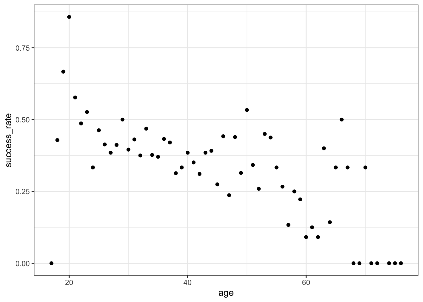
climbers %>%
  mutate(age_bracket = cut(age, breaks = 20)) %>%
  group_by(age_bracket) %>%
  summarize(success_rate = mean(success)) %>%
  ggplot(aes(x = age_bracket, y = success_rate)) +
  geom_point() +
  theme(axis.text.x = element_text(angle = 90, vjust = 0.5, hjust=1))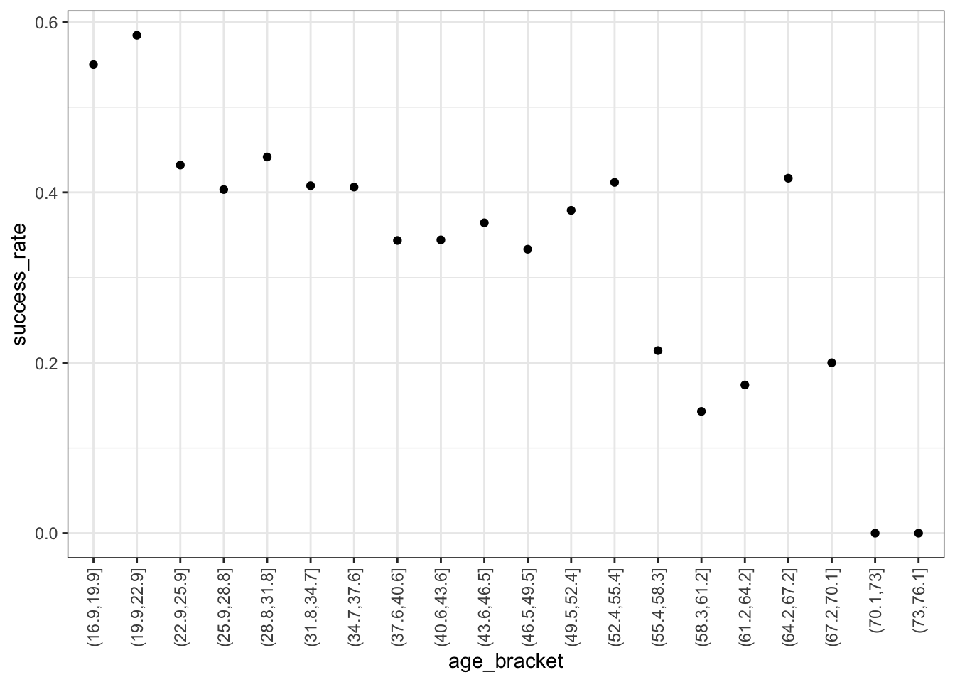
Exercise 3: Logistic regression in R
We’re using glm instead of lm, and add family = "binomial" to specify that this is a logistic model:
climbing_model_1 <- glm(success ~ age, data = climbers, family = "binomial")
coef(summary(climbing_model_1))
##                Estimate  Std. Error   z value     Pr(>|z|)
## (Intercept)  0.42568563 0.169177382  2.516209 1.186249e-02
## age         -0.02397199 0.004489504 -5.339564 9.317048e-08
Exercise 4: Writing out & plotting the model
- .
- log(odds) model
- probability model
- probability model
- odds model
- log(odds) model
Exercise 5: Predictions
#a
log_odds <- 0.42568563 - 0.02397199 * 20
log_odds
## [1] -0.05375417

#b
odds <- exp(log_odds)
odds
## [1] 0.947665

#c
prob <- odds / (odds + 1)
prob
## [1] 0.4865647

#d
predict(climbing_model_1, newdata = data.frame(age = 20))
##           1
## -0.05375421
exp(predict(climbing_model_1, newdata = data.frame(age = 20)))
##        1
## 0.947665
predict(climbing_model_1, newdata = data.frame(age = 20), type = "response")
##         1
## 0.4865647
Exercise 6: Interpreting the intercept
Among 0 year old climbers (lol), the odds of success is 1.5, i.e. 1.5 times more likely than not.
exp(0.42569)
Exercise 7: Interpreting the age coefficient
exp(predict(climbing_model_1, newdata = data.frame(age = 23)))
##         1
## 0.8819057
exp(predict(climbing_model_1, newdata = data.frame(age = 22)))
##         1
## 0.9033021
exp(predict(climbing_model_1, newdata = data.frame(age = 21)))
##         1
## 0.9252177
exp(predict(climbing_model_1, newdata = data.frame(age = 20)))
##        1
## 0.947665
Part a
The odds of success for a 23-year-old are 97.6% as high as those for a 22-year-old (i.e. the odds are 2.4% lower).
0.8819057 / 0.9033021Part b
The odds of success for a 22-year-old are 97.6% as high as those for a 21-year-old (i.e. the odds are 2.4% lower).
0.9033021 / 0.9252177Part c
The odds of success for a 21-year-old are 97.6% as high as those for a 20-year-old (i.e. the odds are 2.4% lower).
0.9252177 / 0.947665Part d
On the log(odds) scale, the
agecoefficient is 0.02397:
On average, for every 1-year increase in age, log(odds of success) decrease by 0.02397.On the odds scale, the
agecoefficient is \(e^{-0.02397} = 0.976313\):
On average, for every 1-year increase in age, odds of success are 97.6% as high. That is, they decrease by 2.4%.
Exercise 8: Another climbing model
# Plot the relationship
climbers %>%
  ggplot(aes(x = oxygen_used, fill = success)) +
  geom_bar(position = "fill")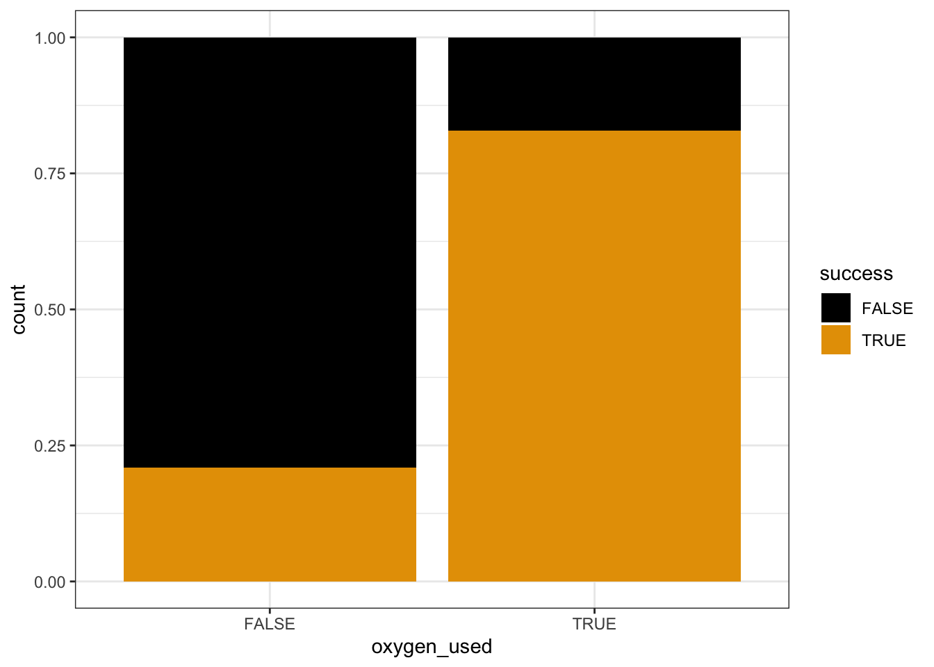
# Model the relationship
climbing_model_2 <- glm(success ~ oxygen_used, data = climbers, family = "binomial")
coef(summary(climbing_model_2))
##                  Estimate Std. Error   z value      Pr(>|z|)
## (Intercept)     -1.327993  0.0639834 -20.75528  1.098514e-95
## oxygen_usedTRUE  2.903864  0.1257404  23.09412 5.304291e-118
Part a
Success is more likely if you use oxygen. The probability of success appears to be between 85% and 90% for people that use oxygen, and under 25% for people that don’t.
Part b
# log(odds)
-1.327993

# odds
exp(-1.327993)

# probability
exp(-1.327993) / (exp(-1.327993) + 1)
Part c
# log(odds)
-1.327993 + 2.903864

# odds
exp(-1.327993 + 2.903864)

# probability
exp(-1.327993 + 2.903864) / (exp(-1.327993 + 2.903864) + 1)
Part d
exp(predict(climbing_model_2, newdata = data.frame(oxygen_used = FALSE)))
##         1
## 0.2650086
predict(climbing_model_2, newdata = data.frame(oxygen_used = FALSE), type = "response")
##         1
## 0.2094915
exp(predict(climbing_model_2, newdata = data.frame(oxygen_used = TRUE)))
##        1
## 4.834951
predict(climbing_model_2, newdata = data.frame(oxygen_used = TRUE), type = "response")
##        1
## 0.828619
Part e
4.834951 / 0.2650086
## [1] 18.24451
Exercise 9: Interpreting coefficients
Part a
This is the odds of success for somebody that doesn’t use oxygen (the reference level).
Part b
This is the odds ratio of success, comparing climbers that use oxygen to those that don’t. The odds of success are 18 times higher if using oxygen.
Exercise 10: Connecting tables to logistic regression
# Rows correspond to oxygen_used
# Columns correspond to success
climbers %>%
  tabyl(oxygen_used, success) %>%
  adorn_totals(c("row", "col"))
##  oxygen_used FALSE TRUE Total
##        FALSE  1166  309  1475
##         TRUE   103  498   601
##        Total  1269  807  2076
Part a
This is the intercept coefficient on the odds scale!
# probability of success (no oxygen)
309 / 1475
## [1] 0.2094915

# odds of success (no oxygen)
(309 / 1475) / (1 - (309 / 1475))
## [1] 0.2650086
Part b
This is the oxygen_usedTRUE coefficient on the odds scale!
# probability of success (oxygen)
498 / 601
## [1] 0.828619

# odds of success (oxygen)
(498 / 601) / (1 - (498 / 601))
## [1] 4.834951

# odds ratio
4.834951 / 0.2650086
## [1] 18.24451