6 Categorical predictors

Announcements etc

SETTLING IN

Sit in your assigned groups, and catch up. This is your last class day in this particular formulation!
Download “06-slr-cat-predictor-notes.qmd”, open it in RStudio, and save it in the “Activities” sub-folder of the “STAT 155” folder.

WRAPPING UP

PP 2 is due tonight.
Nothing is due next week. Study for Quiz 1!!!
Quiz 1 is Thursday (9/25)
- studying
  - check out some study tips in the course manual appendix!
  - there’s a preceptor-led review session on Sunday 1pm-230pm (details on the Moodle calendar)
- structure
  - 60 minutes
  - taken individually, using pen/pencil & paper
- content
  - Unit 1 on Simple Linear Regression, up to and including Thursday’s topic (Categorical predictors). It will not include questions about Transformations.
  - you will not need to write R code, but will need to read & interpret R output
- materials
  - you can use a 3x5 index card with writing on both sides. These can be handwritten or typed, but you may not include screenshots or share note cards – making your own card is important to the review process. You are required to hand this in with your quiz.
  - you cannot use and will not need to use a calculator
- there will be limited opportunities for revision (you can earn up to 50% of missed points back). review syllabus for details.

Learning goals

Write a model formula for a simple linear regression model with a categorical predictor using indicator variables.
Interpret the model coefficients in a simple linear regression model with a categorical predictor.

Additional resources

Required video

Simple linear regression: categorical predictor (slides)

Optional

Watch: R Code for Categorical Predictors
Read: Section 3.9 in the STAT 155 Notes only up through section 3.9.1.

Warm-up

Today we’ll explore penguins!

# Load packages & data
# The penguins data is stored in R
library(tidyverse)
data(penguins)
penguins <- penguins %>% 
  filter(!is.na(sex), !is.na(species))

You can pull up the codebook by typing the following in your CONSOLE: ?penguins

# The cases / units of observation are penguins
# We have data on 333 penguins, 8 variables on each
head(penguins)
dim(penguins)

We’ll focus on 3 variables:

flipper_len = the length of the penguin’s flippers (arms) in mm
species = Adelie, Chinstrap, or Gentoo
sex = female, male

EXAMPLE 1: Get to know the data

# Create a dataset called "chinstraps" that only includes Chinstrap penguins
chinstraps <- penguins %>% 
  ___(species == "Chinstrap")
head(chinstraps)

# Among Chinstraps, what's the average flipper length (mm)?
chinstraps %>% 
  ___(mean(flipper_len))

# Among Chinstraps, how many female and male penguins are there?
# (We haven't used this code in a while!)
chinstraps %>% 
  ___(sex)

EXAMPLE 2: Flipper length vs sex (bad viz)

Among Chinstraps, let’s explore how flipper length might be explained by sex. Use the results below to explain why a scatterplot is not an effective visualization and a line is not an effective summary of the relationship in this example (or for exploring a quantitative Y variable vs categorical X predictor in general).

chinstraps %>% 
  ggplot(aes(y = flipper_len, x = sex)) + 
  geom_point() + 
  geom_smooth(method = "lm", se = FALSE)

EXAMPLE 3: Flipper length vs sex (good viz)

Side-by-side density plots provide a better picture of the relationship between flipper length and sex.

# Check out a density plot of `flipper_len` alone
chinstraps %>% 
  ggplot(aes(x = flipper_len)) + 
  geom_density()

# Modify that code to separate the density plot by sex,
# using different line colors to distinguish females and males:
chinstraps %>% 
  ggplot(aes(x = flipper_len)) + 
  geom_density()

# Modify the code again: use different *fills* to distinguish females and males
chinstraps %>% 
  ggplot(aes(x = flipper_len)) + 
  geom_density()

# Modify this code to create side-by-side *boxplots* of flipper_len by sex
chinstraps %>% 
  ggplot(aes(y = flipper_len)) + 
  geom_boxplot()

# Modify this code to create separate *histograms*:
chinstraps %>% 
  ggplot(aes(x = flipper_len)) + 
  geom_histogram(color = "white") + 
  facet_wrap(~ ___)

FOLLOW-UPS

Describe the relationship of flipper_len with sex.
What do you think was the least effective plot?

Next up: modeling!

We can use linear regression to model the relationship of a quantitative response variable Y with a categorical predictor variable X! This is a relief because predictors are often categorical. Examples:

Model time to campus (Y) by mode of transportation (X) – walk, bike, bus, etc.
Model film revenue (Y) by genre (X) – rom com, sci-fi, etc.
Model wages (Y) by job industry (X) – agriculture, construction, etc.
Model some health outcome (Y) by treatment – A or B.

Though the linear regression model formula is not represented by a line, it still has a familiar form:

$E[Y | X]$ = $\beta_0$ + $\beta_1$ (something related to $X$)

Exercises

Exercise 1: Summaries by category

In exploring the relationship of flipper_len with sex, we’ve explored some visual summaries. Let’s follow these up with some numerical summaries. Recall that among all Chinstraps, males and females combined, the average flipper length was 195.8mm:

chinstraps %>% 
  summarize(mean(flipper_len))

We can calculate separate averages for female and male penguins by adding the group_by() function:

# PAUSE: Note where the group_by() function is, and what information it uses!
chinstraps %>% 
  group_by(sex) %>% 
  summarize(mean(flipper_len))

Part a

Examine the group means, store them in your brain for later, and make sure that you can match these numbers up with what we observed in the plots.

Part b

In the chunk below, calculate the difference between the mean flipper length for male and female penguins (mean for males - mean for females). Check out the actual number and keep this in your brain!

Part c

In general, the group_by() is a unique function in that we’d almost never use it on its own. All it does is change the background structure of the dataset:

# Check out the head of the data set
chinstraps %>% 
  head()

# Check out the head of the data AFTER using group_by
# How did this change?
chinstraps %>% 
  group_by(sex) %>% 
  head()

So we almost always follow up group_by() with summarize():

# Example: calculate the minimum flipper length by sex
chinstraps %>% 
  group_by(sex) %>% 
  summarize(min(flipper_len))

Exercise 2: modeling `flipper_len` by `sex`

Now that we’ve visually and numerically explored the relationship of flipper_len and sex for Chinstrap penguins, let’s build a simple linear regression model of this relationship:

# Construct the model
flipper_model_1 <- lm(flipper_len ~ sex, data = chinstraps)

# Summarize the model
summary(flipper_model_1)

Fill in the resulting model formula:

E[flipper_len | sex] = ___ + ___ sexmale

IMPORTANT: Discuss the following before moving on.

Where have you encountered the 2 model coefficients before?!
Notice that sex shows up as sexmale in the model! This is a 0/1 indicator variable of whether a penguin is male:
- sexmale = 1 if the penguin is male
- sexmale = 0 otherwise (i.e the penguin is female)
In contrast, we do not observe sexfemale in the model output! This is because female is what we call the reference level or reference category of the sex variable. It was chosen to be the reference level simply because, alphabetically, it’s the first sex category. You’ll observe below that female penguins are, indeed, still in the model. You’ll also observe why the term “reference level” makes sense!

Exercise 3: Making sense of the model

Recall our model formula:

E[flipper_len | sex] = 191.735 + 8.176 sexmale

Part a

Use the above model formula to calculate the expected flipper length for a female penguin. HINT: What is sexmale for female penguins, 0 or 1?

191.735 + 8.176 * ___

Part b

Similarly, calculate the expected flipper length for a male penguin.

191.735 + 8.176 * ___

Part c

Re-examine these 2 calculations. Where have you come across these numbers before?!

Exercise 4: Interpreting coefficients

Recall that our model formula is not a formula for a line:

E[flipper_len | sex] = 191.735 + 8.176 sexmale

Thus we can’t interpret the coefficients as we have before when using a quantitative predictor. Taking this into account and reflecting upon your calculations above…

Part a

Interpret the intercept coefficient (191.735) in the penguin context. Make sure to use non-causal language, include units, and talk about averages rather than individual cases.

Part b

Interpret the sexmale coefficient (8.176) in context. Hint: How did you use this value in the prediction calculations above?

Exercise 5: The least squares criterion

The coefficient estimates in this model were selected in the same way as when our predictor is quantitative: by minimizing the sum of the squared residuals.

E[flipper_len | sex] = 191.735 + 8.176 sexmale

Use this model to calculate the residual for the first penguin in the dataset:

# Observed data on the first penguin
chinstraps %>% 
  select(flipper_len, sex) %>% 
  head(1)

Exercise 6: Categorical predictors with >2 categories

Let’s zoom back out to all penguins, not just Chinstraps, and explore how flipper_len can be modeled by species.

# Count up the number of penguins of each species
# (How many species are there?)
penguins %>%

# Construct a side-by-side density plot of the relationship between flipper_len and species

# Calculate the average flipper_len for each species
# Do this without using any filter()!!!

FOLLOW-UP:

Describe what you’ve learned so far about the relationship of flipper_len with species. Be sure to comment on all 3 species!
What is the reference level of the species variable?

Exercise 7: Build & interpret the model

Let’s now model this relationship:

# Construct the model
flipper_model_2 <- lm(flipper_len ~ species, data = penguins)

# Summarize the model
summary(flipper_model_2)

Part a

Complete the model formula below. THINK: Why don’t Adelie penguins show up here?

E[flipper_len | species] = ___ + ___ speciesChinstrap + ___ speciesGentoo

The species related predictors are, again, 0/1 indicator variables:

speciesChinstrap = 1 for Chinstrap penguins and 0 otherwise (for Adelie or Gentoo)
speciesGentoo = 1 for Gentoo penguins and 0 otherwise (for Adelie or Chinstrap)

Part b

Use the model to make some predictions. Use your model formula above, not the predict() function.

# Predict flipper_len for an Adelie penguin


# Predict flipper_len for a Chinstrap penguin


# Predict flipper_len for a Gentoo penguin

Part c

Interpret all 3 model coefficients: 190.1027, 5.7208, 27.1326. Make sure to frame this is context, use non-causal language, include units, and talk about averages rather than individual cases.

Part d

How strong is this model? Since species is a categorical predictor, we cannot use correlation to answer this question – correlation can only be used to measure the strength and direction of a linear relationship between 2 quantitative variables. BUT we can use R-squared.

Report and interpret the R-squared value for flipper_model_2.
Based on this and the fact that flipper_model_1 had an R-squared of 0.33, comment on which is the stronger predictor of flipper_len: species or sex

Exercise 8: Really understand how the coefficients work

Next, consider the model of flipper_len by island. The average flipper_len of penguins on each island is calculated below:

penguins %>% 
  group_by(island) %>% 
  summarize(mean(flipper_len))

Part a

Using just the above averages and your understanding of categorical predictors, fill in the model coefficients and indicator variables below. Do NOT use lm() yet!!!

E[flipper_len | island] = ___ +/- ___ island??? +/- ___ island???

Part b

Check your work to Part a.

flipper_model_3 <- lm(flipper_len ~ island, penguins)
summary(flipper_model_3)

Exercise 9: Diamond price vs color

Load data on diamonds that’s stored in the tidyverse package:

data("diamonds")

# Wrangle the data (don't worry about the code)
diamonds <- diamonds %>% 
    mutate(
        cut = factor(cut, ordered = FALSE),
        color = factor(color, ordered = FALSE),
        clarity = factor(clarity, ordered = FALSE)
    )

head(diamonds)

We’ll explore the relationship between 2 variables:

price of a diamond in USD
color of a diamond, categorized as D (best) through J (worst)

Practice the below steps in order to explore the relationship of diamond price with color.

Before exploring any data, write down what you expect a plot of price vs color to look like. Then construct and interpret an appropriate plot.
Compute the average price for each color. (Remembering the color categories, why is this surprising? What do you think is going on here?)
Fit an appropriate linear model with lm() and display a model summary.
Write out the model formula from the above summary.
Which color is the reference level? How can you tell from the model summary?
Interpret the intercept and two other coefficients from the model in terms of the data context.

Reflection

Through the exercises above, you learned how to build and interpret models that incorporate a categorical predictor variable. For the benefit of your future self, summarize how one can interpret the coefficients for a categorical predictor.

Solutions

# Load packages & data
# The penguins data is stored in R
library(tidyverse)
data(penguins)
penguins <- penguins %>% 
  filter(!is.na(sex), !is.na(species))
dim(penguins)
## [1] 333   8
head(penguins)
##   species    island bill_len bill_dep flipper_len body_mass    sex year
## 1  Adelie Torgersen     39.1     18.7         181      3750   male 2007
## 2  Adelie Torgersen     39.5     17.4         186      3800 female 2007
## 3  Adelie Torgersen     40.3     18.0         195      3250 female 2007
## 4  Adelie Torgersen     36.7     19.3         193      3450 female 2007
## 5  Adelie Torgersen     39.3     20.6         190      3650   male 2007
## 6  Adelie Torgersen     38.9     17.8         181      3625 female 2007

EXAMPLE 1: Get to know the data

# Create a dataset called "chinstraps" that only includes Chinstrap penguins
chinstraps <- penguins %>% 
  filter(species == "Chinstrap")
head(chinstraps)
##     species island bill_len bill_dep flipper_len body_mass    sex year
## 1 Chinstrap  Dream     46.5     17.9         192      3500 female 2007
## 2 Chinstrap  Dream     50.0     19.5         196      3900   male 2007
## 3 Chinstrap  Dream     51.3     19.2         193      3650   male 2007
## 4 Chinstrap  Dream     45.4     18.7         188      3525 female 2007
## 5 Chinstrap  Dream     52.7     19.8         197      3725   male 2007
## 6 Chinstrap  Dream     45.2     17.8         198      3950 female 2007

# Among Chinstraps, what's the average flipper length (mm)?
chinstraps %>% 
  summarize(mean(flipper_len))
##   mean(flipper_len)
## 1          195.8235

# Among Chinstraps, how many female and male penguins are there?
# (We haven't used this code in a while!)
chinstraps %>% 
  count(sex)
##      sex  n
## 1 female 34
## 2   male 34

EXAMPLE 2: Flipper length vs sex (bad viz)

We just have two groups of points (male and female) and it’s tough to identify what’s going on in those groups.
There are so many bad things about modeling this relationship with a line. For one, it suggests that there’s a continuum of observed sex outcomes between male and female.

chinstraps %>% 
  ggplot(aes(y = flipper_len, x = sex)) + 
  geom_point() + 
  geom_smooth(method = "lm", se = FALSE)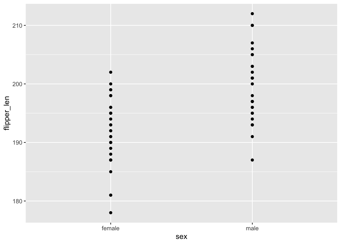

EXAMPLE 3: Flipper length vs sex (good viz)

# Check out a density plot of `flipper_len` alone
chinstraps %>% 
  ggplot(aes(x = flipper_len)) + 
  geom_density()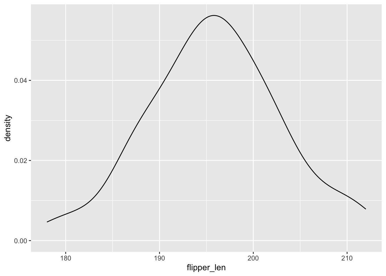


# Modify that code to separate the density plot by sex,
# using different line colors to distinguish females and males:
chinstraps %>% 
  ggplot(aes(x = flipper_len, color = sex)) + 
  geom_density()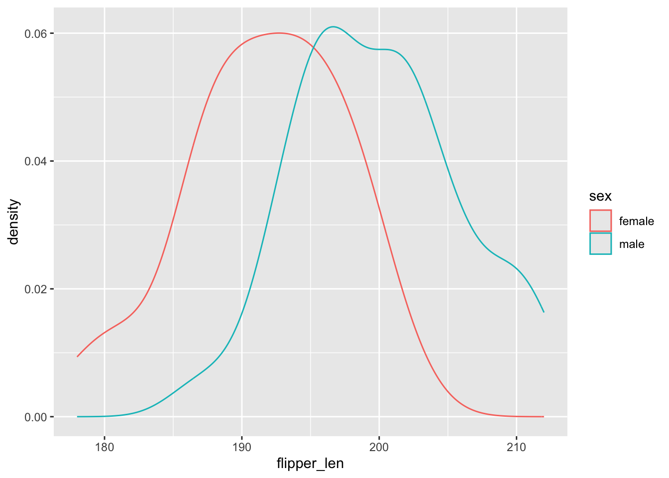


# Modify the code again: use different *fills* to distinguish females and males
chinstraps %>% 
  ggplot(aes(x = flipper_len, fill = sex)) + 
  geom_density(alpha = 0.5)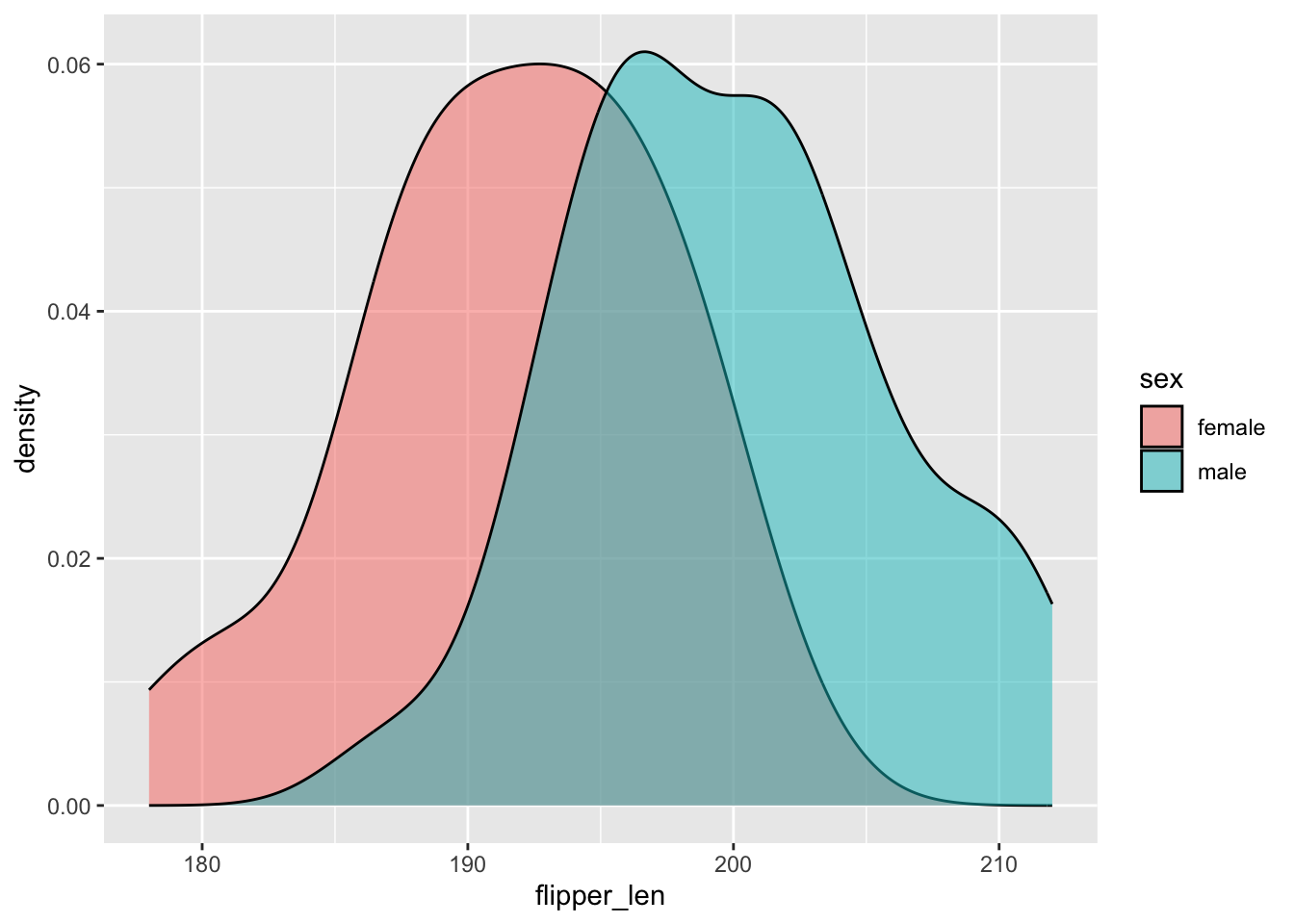


# Modify this code to create side-by-side *boxplots* of flipper_len by sex
chinstraps %>% 
  ggplot(aes(y = flipper_len, x = sex)) + 
  geom_boxplot()


chinstraps %>% 
  ggplot(aes(x = flipper_len)) + 
  geom_histogram(color = "white") + 
  facet_wrap(~ sex)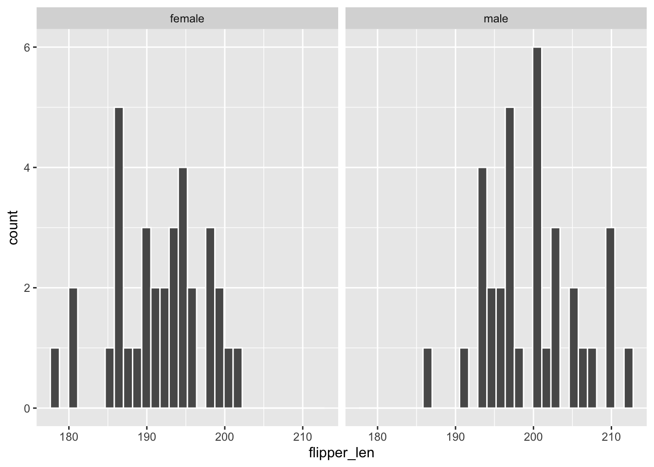

FOLLOW-UPS

Flipper lengths are similarly variable among female and male penguins, though male penguins tend to have longer flippers. The typical flipper length is ~200mm among males and ~192mm among females.
The histograms are tough to compare.

Exercise 1: Summaries by category

chinstraps %>% 
  summarize(mean(flipper_len))
##   mean(flipper_len)
## 1          195.8235

chinstraps %>% 
  group_by(sex) %>% 
  summarize(mean(flipper_len))
## # A tibble: 2 × 2
##   sex    `mean(flipper_len)`
##   <fct>                <dbl>
## 1 female                192.
## 2 male                  200.

# Difference in mean flipper length for male and female penguins
200 - 192
## [1] 8

Exercise 2: modeling `flipper_len` by `sex`

# Construct the model
flipper_model_1 <- lm(flipper_len ~ sex, data = chinstraps)

# Summarize the model
summary(flipper_model_1)
## 
## Call:
## lm(formula = flipper_len ~ sex, data = chinstraps)
## 
## Residuals:
##      Min       1Q   Median       3Q      Max 
## -13.7353  -4.1176   0.2647   3.5147  12.0882 
## 
## Coefficients:
##             Estimate Std. Error t value Pr(>|t|)    
## (Intercept)  191.735      1.006 190.577  < 2e-16 ***
## sexmale        8.176      1.423   5.747 2.53e-07 ***
## ---
## Signif. codes:  0 '***' 0.001 '**' 0.01 '*' 0.05 '.' 0.1 ' ' 1
## 
## Residual standard error: 5.866 on 66 degrees of freedom
## Multiple R-squared:  0.3335, Adjusted R-squared:  0.3234 
## F-statistic: 33.02 on 1 and 66 DF,  p-value: 2.526e-07

E[flipper_len | sex] = 191.735 + 8.176 sexmale

191.735 is similar to the mean calculation for females
8.176 is similar to the difference in mean calculations (male - female)

Exercise 3: Making sense of the model

Part a

191.735 + 8.176*0
## [1] 191.735

Part b

191.735 + 8.176*1
## [1] 199.911

Part c

These are the mean flipper lengths by sex:

chinstraps %>% 
  group_by(sex) %>% 
  summarize(mean(flipper_len))

Exercise 4: Interpreting coefficients

Part a

191.735 is the average / expected flipper length among female penguins (i.e. when sexmale is 0).

Part b

The average flipper length among male penguins is 8.176mm bigger than that of female penguins.

NOTE: This isn’t a slope, but does tell us about the change in the average flipper length when we increase the sexmale predictor by 1 – here that means going from sexmale = 0 (female) to sexmale = 1 (male).

Exercise 5: The least squares criterion

# Observed Y 
192
## [1] 192

# Predicted Y (based on the penguin being female)
191.735 + 8.176*0
## [1] 191.735

# Residual
192 - 191.735
## [1] 0.265

Exercise 6: Categorical predictors with >2 categories

# Count up the number of penguins of each species
# (How many species are there?)
penguins %>% 
  count(species)

# Construct a side-by-side density plot of the relationship
# between flipper_len and species
penguins %>% 
  ggplot(aes(x = flipper_len, color = species)) + 
  geom_density()

# Calculate the average flipper_len for each species
# Do this without using any filter()!!!
penguins %>% 
  group_by(species) %>% 
  summarize(mean(flipper_len))

FOLLOW-UP:

Flipper lengths are similarly variable within each species. Gentoos tend to have the longest flippers and Adelie the shortest. Chinstraps are in between and tend to have slightly longer flippers than Adelie.
reference level is Adelie, the first alphabetically

Exercise 7: Build & interpret the model

# Construct the model
flipper_model_2 <- lm(flipper_len ~ species, data = penguins)

# Summarize the model
summary(flipper_model_2)
## 
## Call:
## lm(formula = flipper_len ~ species, data = penguins)
## 
## Residuals:
##      Min       1Q   Median       3Q      Max 
## -18.1027  -4.8235  -0.1027   4.7647  19.8973 
## 
## Coefficients:
##                  Estimate Std. Error t value Pr(>|t|)    
## (Intercept)      190.1027     0.5522  344.25  < 2e-16 ***
## speciesChinstrap   5.7208     0.9796    5.84 1.25e-08 ***
## speciesGentoo     27.1326     0.8241   32.92  < 2e-16 ***
## ---
## Signif. codes:  0 '***' 0.001 '**' 0.01 '*' 0.05 '.' 0.1 ' ' 1
## 
## Residual standard error: 6.673 on 330 degrees of freedom
## Multiple R-squared:  0.7747, Adjusted R-squared:  0.7734 
## F-statistic: 567.4 on 2 and 330 DF,  p-value: < 2.2e-16

Part a

E[flipper_len | species] = 190.1027 + 5.7208 speciesChinstrap + 27.1326 speciesGentoo

Part b

# Predict flipper_len for an Adelie penguin
190.1027 + 5.7208*0 + 27.1326*0
## [1] 190.1027

# Predict flipper_len for a Chinstrap penguin
190.1027 + 5.7208*1 + 27.1326*0
## [1] 195.8235

# Predict flipper_len for a Gentoo penguin
190.1027 + 5.7208*0 + 27.1326*1
## [1] 217.2353

Part c

190.10 is the average flipper length among Adelie penguins (i.e. when speciesChinstrap and speciesGentoo are both 0).
The average flipper length among Chinstrap penguins is 5.72mm bigger than that of Adelie penguins.
The average flipper length among Gentoo penguins is 27.13mm bigger than that of Adelie penguins.

Part d

This model of flipper_len by species explains roughly 77% of the variability in flipper length from penguin to penguin.

Exercise 8: Really understand how the coefficients work

penguins %>% 
  group_by(island) %>% 
  summarize(mean(flipper_len))
## # A tibble: 3 × 2
##   island    `mean(flipper_len)`
##   <fct>                   <dbl>
## 1 Biscoe                   210.
## 2 Dream                    193.
## 3 Torgersen                192.

Part a

E[flipper_len | island] = 209.56 - 16.37 islandDream - 18.03 islandTorgersen

Why?

The island terms are islandDream and islandTorgersen since Biscoe is the reference.
The intercept is the average flipper length for the reference, Biscoe.
The islandDream coefficient reflects the fact that the average flipper length on Dream is 16.37mm lower than that on Biscoe (193.1870 - 209.5583)
The islandTorgersen coefficient reflects the fact that the average flipper length on Dream is 18.03mm lower than that on Biscoe (191.5319 - 209.5583)

Part b

flipper_model_3 <- lm(flipper_len ~ island, penguins)
summary(flipper_model_3)
## 
## Call:
## lm(formula = flipper_len ~ island, data = penguins)
## 
## Residuals:
##     Min      1Q  Median      3Q     Max 
## -37.558  -5.532   1.468   7.442  21.442 
## 
## Coefficients:
##                 Estimate Std. Error t value Pr(>|t|)    
## (Intercept)      209.558      0.879 238.410   <2e-16 ***
## islandDream      -16.371      1.340 -12.214   <2e-16 ***
## islandTorgersen  -18.026      1.858  -9.702   <2e-16 ***
## ---
## Signif. codes:  0 '***' 0.001 '**' 0.01 '*' 0.05 '.' 0.1 ' ' 1
## 
## Residual standard error: 11.22 on 330 degrees of freedom
## Multiple R-squared:  0.3628, Adjusted R-squared:  0.3589 
## F-statistic: 93.94 on 2 and 330 DF,  p-value: < 2.2e-16

Exercise 9: Diamond price vs color

data("diamonds")

# Wrangle the data (don't worry about the code)
diamonds <- diamonds %>% 
    mutate(
        cut = factor(cut, ordered = FALSE),
        color = factor(color, ordered = FALSE),
        clarity = factor(clarity, ordered = FALSE)
    )

head(diamonds)
## # A tibble: 6 × 10
##   carat cut       color clarity depth table price     x     y     z
##   <dbl> <fct>     <fct> <fct>   <dbl> <dbl> <int> <dbl> <dbl> <dbl>
## 1  0.23 Ideal     E     SI2      61.5    55   326  3.95  3.98  2.43
## 2  0.21 Premium   E     SI1      59.8    61   326  3.89  3.84  2.31
## 3  0.23 Good      E     VS1      56.9    65   327  4.05  4.07  2.31
## 4  0.29 Premium   I     VS2      62.4    58   334  4.2   4.23  2.63
## 5  0.31 Good      J     SI2      63.3    58   335  4.34  4.35  2.75
## 6  0.24 Very Good J     VVS2     62.8    57   336  3.94  3.96  2.48

The best color diamonds are J, and worst are D. We would expect D diamonds to have the lowest price and increase steadily as we get to J. This is in fact what we see in the boxplots.

ggplot(diamonds, aes(x = color, y = price)) +
  geom_boxplot()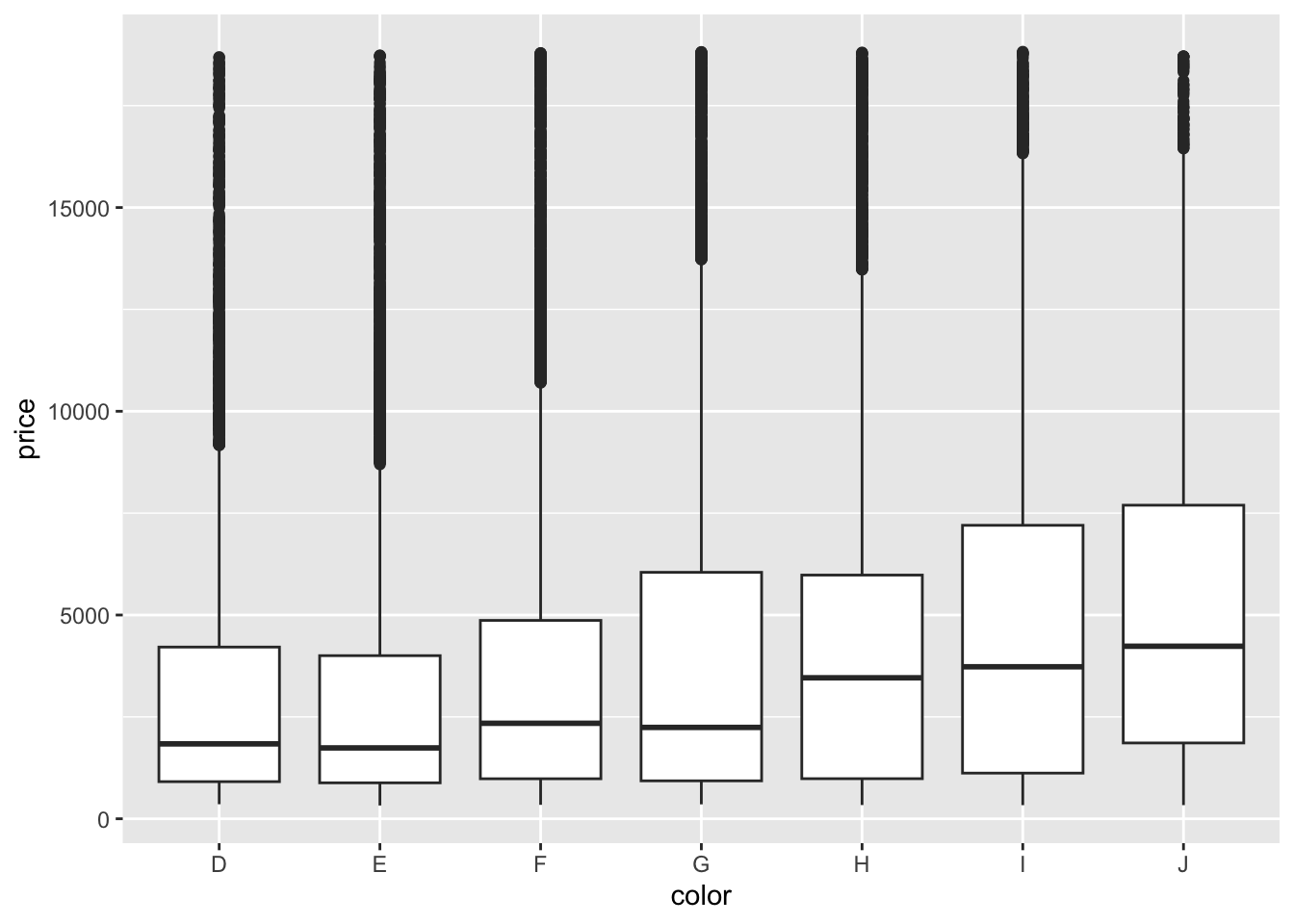


diamonds %>% 
  group_by(color) %>% 
  summarize(mean(price))
## # A tibble: 7 × 2
##   color `mean(price)`
##   <fct>         <dbl>
## 1 D             3170.
## 2 E             3077.
## 3 F             3725.
## 4 G             3999.
## 5 H             4487.
## 6 I             5092.
## 7 J             5324.

We fit a linear model and obtain the model formula: E[price | color] = 3169.95 - 93.20 colorE + 554.93 colorF + 829.18 colorG + 1316.72 colorH + 1921.92 colorI + 2153.86 colorJ

diamond_mod2 <- lm(price ~ color, data = diamonds)

coef(summary(diamond_mod2))
##               Estimate Std. Error   t value      Pr(>|t|)
## (Intercept) 3169.95410   47.70694 66.446391  0.000000e+00
## colorE       -93.20162   62.04724 -1.502107  1.330752e-01
## colorF       554.93230   62.38527  8.895246  6.004834e-19
## colorG       829.18158   60.34470 13.740751  6.836340e-43
## colorH      1316.71510   64.28715 20.481777  7.074714e-93
## colorI      1921.92086   71.55308 26.860072 7.078041e-158
## colorJ      2153.86392   88.13203 24.439060 3.414906e-131

Color D is the reference level because we don’t see its indicator variable in the model output.
Interpretation of the intercept: Diamonds with D color cost $3169.95 on average.
Interpretation of the colorE coefficient: Diamonds with E color cost $93.20 less than D color diamonds on average.
Interpretation of the colorF coefficient: Diamonds with F color cost $554.93 more than D color diamonds on average.

Announcements etc

Warm-up

Exercises

Exercise 1: Summaries by category

Part a

Part b

Part c

Exercise 2: modeling flipper_len by sex

Exercise 3: Making sense of the model

Part a

Part b

Part c

Exercise 4: Interpreting coefficients

Part a

Part b

Exercise 5: The least squares criterion

Exercise 6: Categorical predictors with >2 categories

Exercise 7: Build & interpret the model

Part a

Part b

Part c

Part d

Exercise 8: Really understand how the coefficients work

Part a

Part b

Exercise 9: Diamond price vs color

Reflection

Solutions

Exercise 1: Summaries by category

Exercise 2: modeling flipper_len by sex

Exercise 3: Making sense of the model

Part a

Part b

Part c

Exercise 4: Interpreting coefficients

Part a

Part b

Exercise 5: The least squares criterion

Exercise 6: Categorical predictors with >2 categories

Exercise 7: Build & interpret the model

Part a

Part b

Part c

Part d

Exercise 8: Really understand how the coefficients work

Part a

Part b

Exercise 9: Diamond price vs color

Exercise 2: modeling `flipper_len` by `sex`

Exercise 2: modeling `flipper_len` by `sex`