library(tidyverse)
data(penguins)
gentoo <- penguins %>%
  filter(species == "Gentoo")
dim(gentoo)17 Sampling distribution recap + project time
Announcements etc
SETTLING IN
- Find the qmd here: “17-sampling-recap-projects-notes.qmd”.
WRAPPING UP
Upcoming due dates:
TODAY: Project Milestone 1
Use the template and directions on Moodle!Next week
- Tuesday
- Quiz 2 revisions (at the start of class)
Follow the directions on Moodle! If you follow directions, you can get up to 50% of points back. If you don’t follow directions, you can get up to 33% of points back. - CP 14
- Quiz 2 revisions (at the start of class)
- Thursday
- PP 6
- Tuesday
Related but unrelated: MSCS events calendar
Warm-up
CONTEXT
We want to make inferences about the relationship of body mass with flipper length among Gentoo penguins:
E[body_mass | flipper_len] = \(\beta_0\) + \(\beta_1\) flipper_len
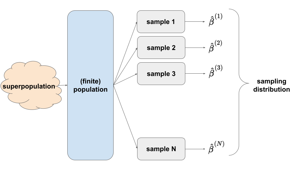
POPULATION vs SAMPLE
Superpopulation = underlying process that governs the relationship of body mass with flipper length among all Gentoo penguins that have ever been, are, and will be!
(Finite) population = at the time the data was collected, all Gentoo penguins that existed
Sample = the 124 Gentoo penguins in our sample
WHAT’S NEXT
Ours is one of many samples we might have gotten.
There’s error in using this sample to estimate features of the broader population.
We must gain a sense of just how much error there might be.
Sampling distributions can provide insight into this sampling variability and standard errors.
- We can approximate features of the sampling distribution using
- Central Limit Theorem (CLT)
- formula-based approach: assumes Normality of different sample estimates \(\hat{\beta}\)
- The quality of this approximation hinges upon the validity of the Central Limit Theorem which hinges upon the validity of the theoretical model assumptions, as well as a “large enough” sample size n.
- The CLT uses theoretical formulas for the standard error estimates, thus can feel a little mysterious without a solid foundation in probability theory.
- BUT: When the theory is “valid”, nothing beats a CLT approximation!!!
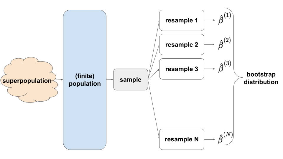
- bootstrapping
- simulation-based approach: exploring different REsamples from our sample provides insight into the behavior of different samples from the population (hence features of the sampling distribution)
- The statistical theory behind bootstrapping is quite complicated, and there are certain obscure cases (none that we will encounter in STAT 155) where the assumptions underlying bootstrapping fail to hold.
- It cannot and should not replace the CLT. BUT, it but gives us some nice intuition behind the idea of resampling, which is fundamental for hypothesis testing (which we’ll get to shortly!).
- simulation-based approach: exploring different REsamples from our sample provides insight into the behavior of different samples from the population (hence features of the sampling distribution)
- Central Limit Theorem (CLT)
EXAMPLE 1: CLT
penguin_sample_mod <- lm(body_mass ~ flipper_len, gentoo)
coef(summary(penguin_sample_mod))

gentoo %>%
  ggplot(aes(y = body_mass, x = flipper_len)) +
  geom_point() +
  geom_smooth(method = "lm", se = FALSE)
Our sample estimate of \(\beta_1\) is \(\hat{\beta}_1 = 54.62\). There’s error in this estimate!!! For samples of 124 penguins, what’s the typical error in using that sample to estimate \(\beta_1\)? That is, what’s the typical difference between \(\hat{\beta}_1\) and \(\beta_1\)?
We can approximate the sampling distribution of \(\hat{\beta}_1\) using the CLT. Sketch the CLT (on paper), along with markings representing the 68-95-99.7 Rule. REMEMBER: This is the assumed model of all possible \(\hat{\beta}_1\) sample estimates we might get from all possible samples of 124 penguins (not just the one sample we happened to get).
EXAMPLE 2: Applying the CLT
Our sample estimate was \(\hat{\beta}_1 = 54.62\).
What’s the chance that our estimate is within 5.03 units (g/cm) of the actual \(\beta_1\)?
What’s the chance that our estimate is within 10.06 units (g/cm) of the actual \(\beta_1\)?
What’s the chance that our estimate is more than 10.06 units (g/cm) from the actual \(\beta_1\)?
What’s the chance that our estimate is more than 10.06 units (g/cm) above the actual \(\beta_1\)?
EXAMPLE 3: Bootstrapping
Obtain 500 bootstrap estimates of the population flipper_len coefficient \(\beta_1\):
# Set the seed so that we all get the same results
set.seed(155)

# Store the sample models
boot_models <- mosaic::___(___)*(
  gentoo %>%
    ___(size = ___, replace = ___) %>%
    with(___(body_mass ~ flipper_len))
)

# Check out the first 6 results
head(boot_models)
Plot the 500 sample model lines. The red line represents the model estimate calculated from our original sample of 124 penguins (not the population model, which we don’t know!):
gentoo %>%
  ggplot(aes(x = flipper_len, y = body_mass)) +
  geom_smooth(method = "lm", se = FALSE) +
  geom_abline(data = boot_models,
              aes(intercept = Intercept, slope = flipper_len),
              color = "gray", size = 0.25) +
  geom_smooth(method = "lm", color = "red", se = FALSE)
Plot the 500 bootstrap slopes. This approximates features of the sampling distribution of \(\hat{\beta}_1\). The red line represents the slope estimate calculated from our original sample of 124 penguins:
boot_models %>%
  ggplot(aes(x = flipper_len)) +
  geom_density() +
  geom_vline(xintercept = 54.62, color = "red")
Use the bootstrap estimates to approximate the standard error of \(\hat{\beta}_1\). Is this consistent with the standard error of 5.03 as calculated via a formula and reported in the model summary table?!
boot_models %>%
  ___(___(flipper_len))
EXAMPLE 4: Connecting new and old ideas
Our sample model is plotted below, using geom_smooth() without se = FALSE. Discuss!
gentoo %>%
  ggplot(aes(y = body_mass, x = flipper_len)) +
  geom_smooth(method = "lm")
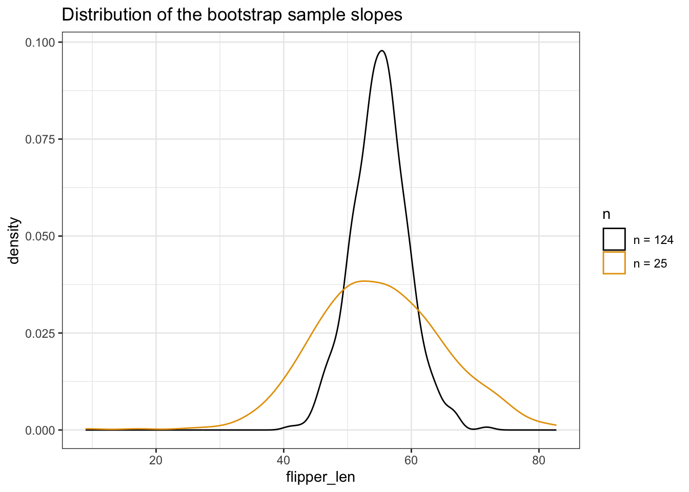
EXAMPLE 5: Impact of sample size
Using the plots below, discuss the impact of sample size n on the sampling distribution and standard error of \(\hat{\beta}_1\).
# DO NOT WORRY ABOUT THIS CODE!!!

# Set the seed so that we all get the same results
set.seed(155)

# Store the sample models
boot_models_small <- mosaic::do(500)*(
  gentoo %>%
    sample_n(size = 25, replace = TRUE) %>%
    with(lm(body_mass ~ flipper_len))
)

boot_combo <- rbind(boot_models, boot_models_small) %>%
  mutate(n = rep(c("n = 124", "n = 25"), each = 500))

gentoo %>%
  ggplot(aes(x = flipper_len, y = body_mass)) +
  geom_smooth(method = "lm", se = FALSE) +
  geom_abline(data = boot_combo, aes(intercept = Intercept, slope = flipper_len),
              color = "gray", size = 0.25) +
  geom_smooth(method = "lm", color = "red", se = FALSE) +
  facet_wrap(~ n) +
  labs(title = "Bootstrap sample models")
# DO NOT WORRY ABOUT THIS CODE!!!
boot_combo %>%
ggplot(aes(x = flipper_len, color = n)) +
geom_density() +
labs(title = "Distribution of the bootstrap sample slopes")
Project time
EXPECTATIONS
You should be working together on your project. If you’re not, then you are neither engaged in class (an expectation for the class itself) nor the collaboration (an expectation for your project).
Make the most of your time together in class! Time is precious and it will be tough to find a time that you can all meet outside class.
Support one another! One goal of this project is independence (from the instructor, not your group :)).
- If you have a question about code / concepts, first ask your group.
- If your group can’t figure it out, your group should ask Google (this is a skill!).
- If you’re still stumped, then talk to the instructor. They can give you a nudge, but not the answer.
Your final project grade will reflect your individual engagement and contributions to the project. You are not expected to be perfect. Rather, you should put effort, attention, and reflection into the following areas:
- contributing to group discussions
- including all other group members in discussion
- creating a space where others felt comfortable sharing ideas and mistakes
- communicating with your group outside class
- contributing to the content / analysis in the report
- contributing to the writing of the report
- contributing to the editing of the report
DIRECTIONS
Discuss your Milestone 1 with group mates.
Each student should take ~5 minutes to showcase what you’ve explored thus far:- Share your research questions. Show and discuss your plots.
- Have you discovered anything interesting? Uninteresting?
- If you continued digging into your research question, what follow-up questions would you have? What would be the next step?
Wrap up Project Milestone 1 (due today!).
Start thinking about Project Milestone 2!! Directions are in the Final project info & description doc.
Solutions
data(penguins)
gentoo <- penguins %>%
filter(species == "Gentoo")
dim(gentoo)
## [1] 124 8EXAMPLE 1: CLT
penguin_sample_mod <- lm(body_mass ~ flipper_len, gentoo)
coef(summary(penguin_sample_mod))
## Estimate Std. Error t value Pr(>|t|)
## (Intercept) -6787.2806 1092.551940 -6.212318 7.649742e-09
## flipper_len 54.6225 5.028244 10.863137 1.330279e-19
gentoo %>%
ggplot(aes(y = body_mass, x = flipper_len)) +
geom_point() +
geom_smooth(method = "lm", se = FALSE)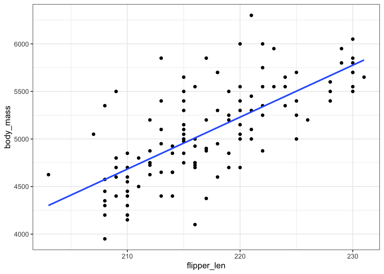
5.03 g/cm
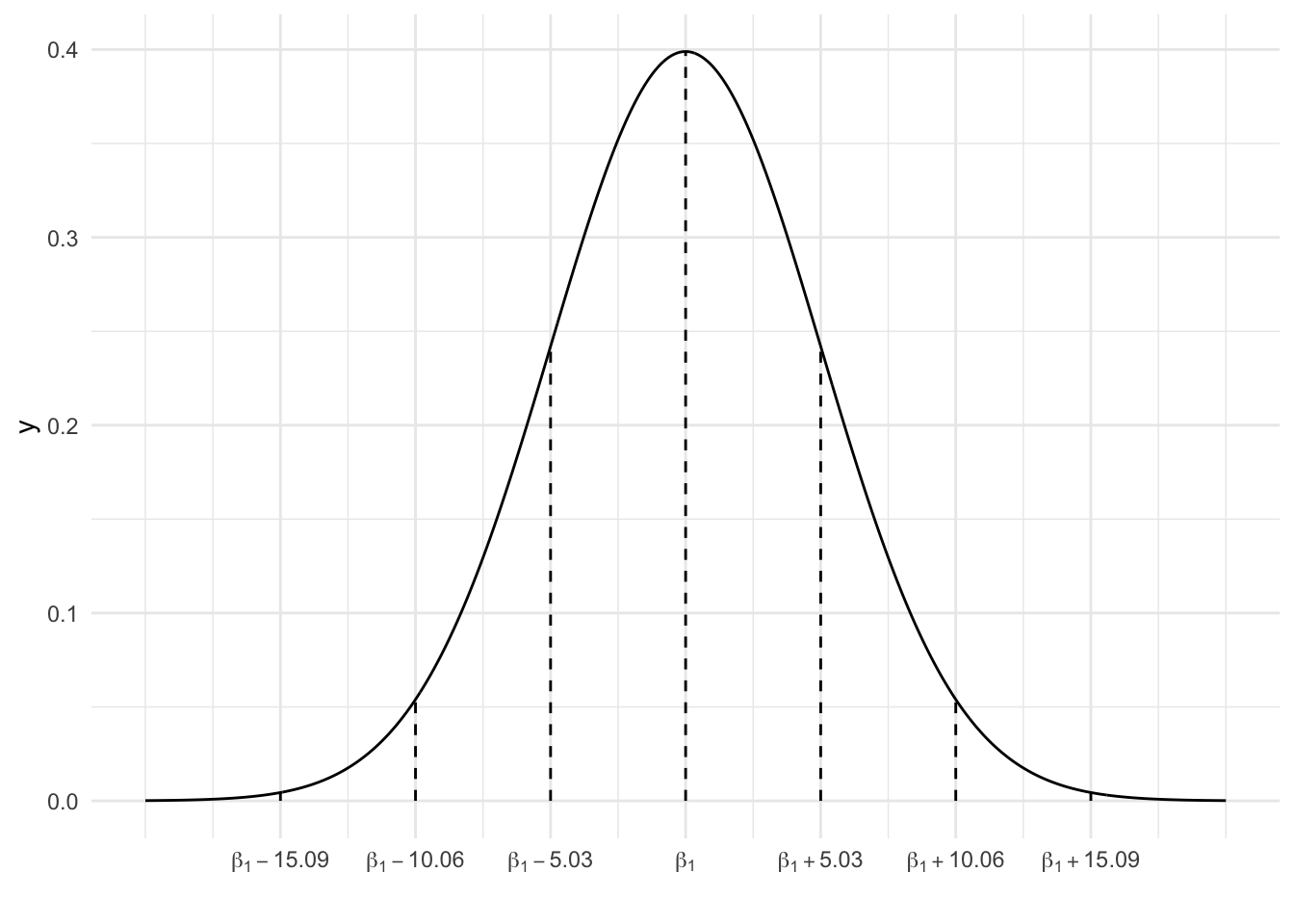
EXAMPLE 2: Applying the CLT
- 68% (68% of samples produce estimates within 1 s.e. of \(\beta_1\))
- 95% (95% of samples produce estimates within 2 s.e. of \(\beta_1\))
- 5% (Since 95% of estimates are within 2 s.e. of \(\beta_1\), 5% are more than 2 s.e. away)
- 2.5% (Since 5% of estimates are more than 2 s.e. away…2.5% are more than 2 s.e. above \(\beta_1\) and 2.5% are more than 2 s.e. below \(\beta_1\))
EXAMPLE 3: Bootstrapping
# Set the seed so that we all get the same results
set.seed(155)
# Store the sample models
boot_models <- mosaic::do(500)*(
gentoo %>%
sample_n(size = 124, replace = TRUE) %>%
with(lm(body_mass ~ flipper_len))
)
# Check out the first 6 results
head(boot_models)
## Intercept flipper_len sigma r.squared F numdf dendf .row .index
## 1 -7244.446 56.80923 365.6557 0.4824797 111.8749 1 120 1 1
## 2 -6234.333 52.07017 376.5489 0.4902570 115.4127 1 120 1 2
## 3 -7053.273 55.69311 346.2286 0.4799553 111.6723 1 121 1 3
## 4 -7297.143 56.82195 360.5165 0.5421990 143.3070 1 121 1 4
## 5 -7166.544 56.40986 375.5472 0.4892053 116.8435 1 122 1 5
## 6 -6135.910 51.62211 334.6243 0.5045329 124.2323 1 122 1 6
# Plot the 500 sample model lines.
# The *red line* represents the model estimate calculated from our *original* sample of 124 penguins (not the population model, which we don't know!)
gentoo %>%
ggplot(aes(x = flipper_len, y = body_mass)) +
geom_smooth(method = "lm", se = FALSE) +
geom_abline(data = boot_models,
aes(intercept = Intercept, slope = flipper_len),
color = "gray", size = 0.25) +
geom_smooth(method = "lm", color = "red", se = FALSE)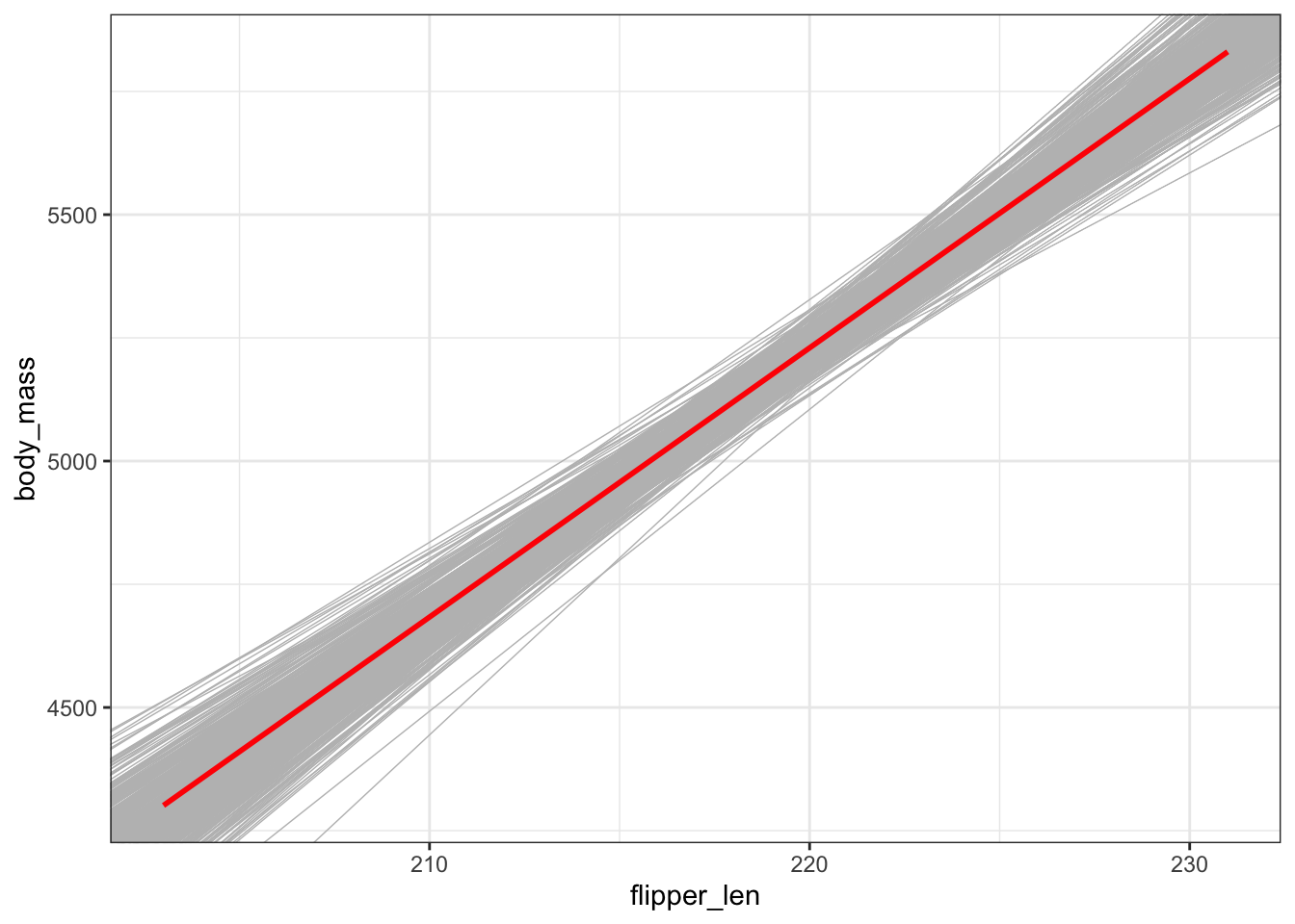
# Plot the 500 bootstrap slopes.
# This *approximates* features of the **sampling distribution** of $\hat{\beta}_1$.
# The *red line* represents the slope estimate calculated from our *original* sample of 124 penguins:
boot_models %>%
ggplot(aes(x = flipper_len)) +
geom_density() +
geom_vline(xintercept = 54.62, color = "red")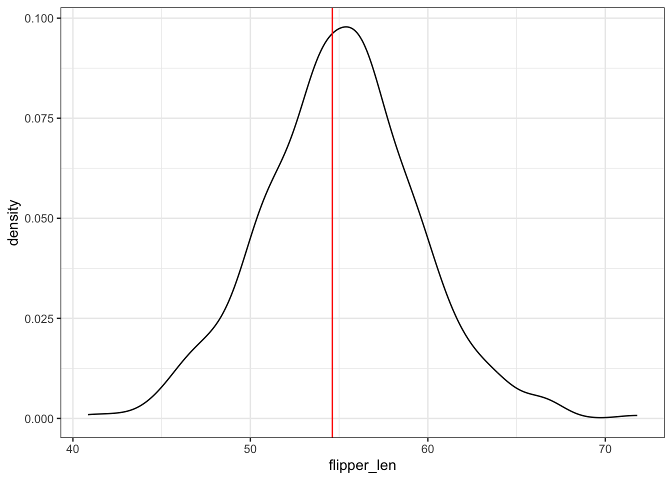
#Use the bootstrap estimates to *approximate* the standard error of our sample slope
boot_models %>%
summarize(sd(flipper_len))
## sd(flipper_len)
## 1 4.341151
EXAMPLE 4: Connecting new and old ideas
This “confidence band” obtained via CLT assumptions is consistent with our bootstrap sample models. It reflects the potential error in our overall sample model.
gentoo %>%
ggplot(aes(y = body_mass, x = flipper_len)) +
geom_smooth(method = "lm")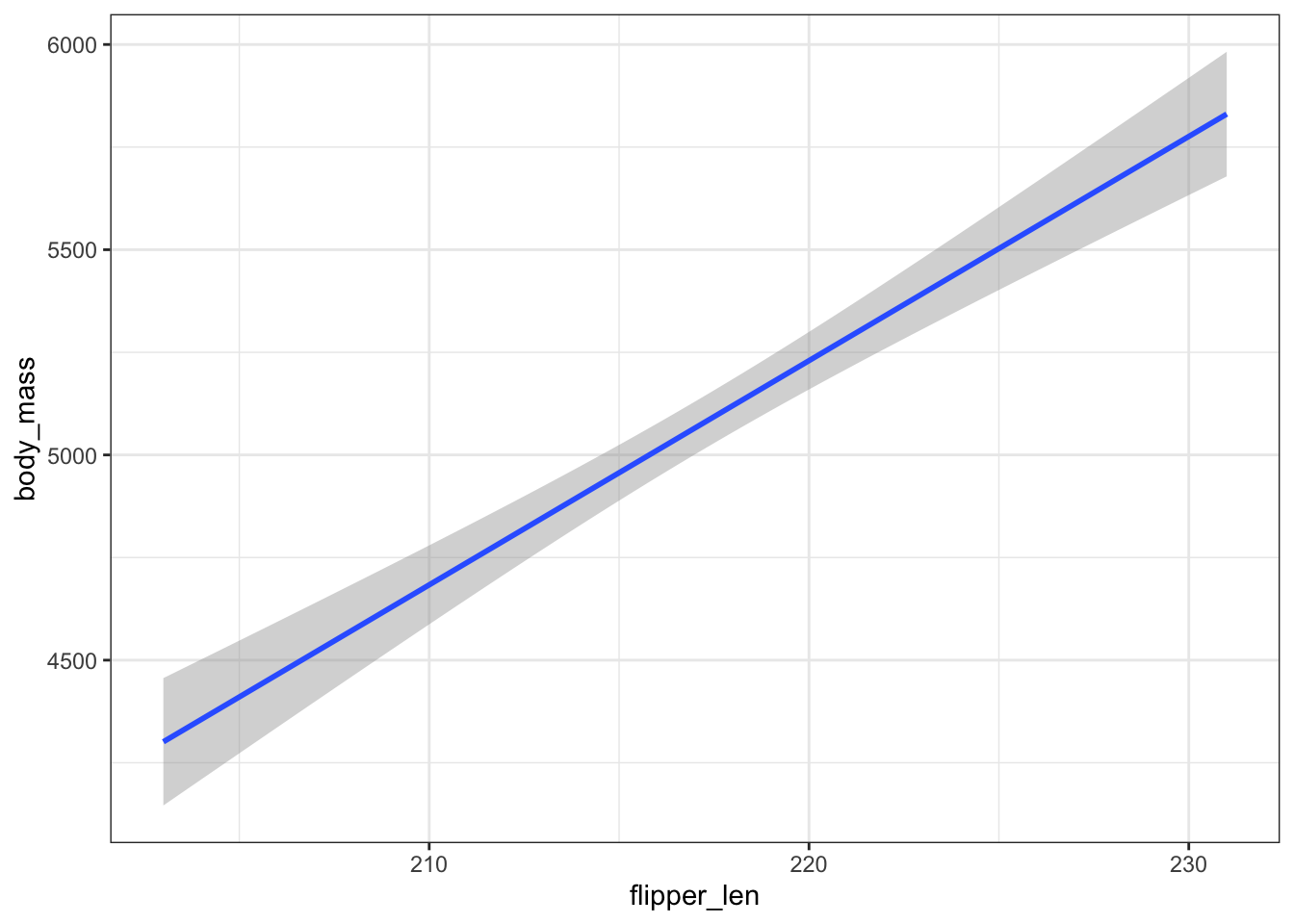
EXAMPLE 5: Impact of sample size
As long as n is big enough, the sample estimates will be normally distributed around \(\beta_1\). But the bigger the sample size, the smaller the sampling variability (the more similar the sample models) hence the smaller the standard error in the sample slope estimates:
# DO NOT WORRY ABOUT THIS CODE!!!
# Set the seed so that we all get the same results
set.seed(155)
# Store the sample models
boot_models_small <- mosaic::do(500)*(
gentoo %>%
sample_n(size = 25, replace = TRUE) %>%
with(lm(body_mass ~ flipper_len))
)
boot_combo <- rbind(boot_models, boot_models_small) %>%
mutate(n = rep(c("n = 124", "n = 25"), each = 500))
gentoo %>%
ggplot(aes(x = flipper_len, y = body_mass)) +
geom_smooth(method = "lm", se = FALSE) +
geom_abline(data = boot_combo, aes(intercept = Intercept, slope = flipper_len),
color = "gray", size = 0.25) +
geom_smooth(method = "lm", color = "red", se = FALSE) +
facet_wrap(~ n) +
labs(title = "Bootstrap sample models")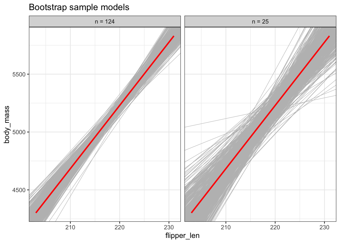
# DO NOT WORRY ABOUT THIS CODE!!!

boot_combo %>%
  ggplot(aes(x = flipper_len, color = n)) +
  geom_density() +
  labs(title = "Distribution of the bootstrap sample slopes")