11 Model building

Announcements etc

SETTLING IN

Put away phones (in your backpack, not face down on your table).
Due now: Quiz 1 revisions
Get ready to take notes: “11-mlr-model-building-notes.qmd”.

WRAPPING UP

Between now and our next class: finish your activity and study (review recent material).
Upcoming due dates:
- Next Tuesday = PP 4 and CP 10

Learning goals

Distinguish between descriptive, predictive, and causal research questions.
Understand when variables are redundant or multicollinear, as well as the corresponding impact on coefficient estimates and \(R^2\).
Explain why adjusted \(R^2\) is preferable to multiple \(R^2\) when comparing models with different numbers of predictors.

Additional resources

Required video

Causal Diagrams and Confounding Variables

Optional

Read: Section 3.9.5 in the STAT 155 Notes
Watch: Redundancy and Multicollinearity

Warm-up

OPTIONAL Math Box: Fitting multiple linear regression models

Consider a multiple linear regression model with \(p\) predictors:

\[E[Y|X_1,X_2,...,X_p] = \beta_0 + \beta_1 X_1 + \beta_2 X_2 + ... + \beta_p X_p\]

We use the least squares criterion to estimate \((\beta_0, \beta_1, ..., \beta_p)\), i.e. we pick the coefficients minimize the sum of squared residuals. Just as with simple linear regression, we can write out a formula for these least square estimates. But for multiple linear regression, this requires linear algebra.

Suppose we have \(n\) data points. Using matrix notation, we can collect our observed response values into a vector \(Y\), our predictor values into a matrix \(X\), and our regression coefficients into a vector \(\beta\). The column of 1s in \(X\) reflects our model’s inclusion of an intercept:

\[Y = \left(\begin{array}{c} Y_1 \\ Y_2 \\ \vdots \\ Y_n \end{array} \right) \;\;\;\; \text{ and } \;\;\;\; X = \left(\begin{array}{ccccc} 1 & X_{11} & X_{12} & \cdots & X_{1p} \\ 1 & X_{21} & X_{22} & \cdots & X_{2p} \\ \vdots & \vdots & \vdots & \cdots & \vdots \\ 1 & X_{n1} & X_{n2} & \cdots & X_{np} \\ \end{array} \right) \;\;\;\; \text{ and } \;\;\;\; \beta = \left(\begin{array}{c} \beta_0 \\ \beta_1 \\ \vdots \\ \beta_p \end{array} \right)\]

Then we can express the model \(E[Y_i|X_{i1}, X_{i2},...,X_{ip}] = \beta_0 + \beta_1 X_{i1} + \cdots + \beta_p X_{ip}\) for \(i \in \{1,...,n\}\) as:

\[E[Y|X] = X\beta\] Further, let \(\hat{\beta}\) denote the vector of sample estimated \(\beta\) and \(\hat{Y}\) denote the vector of predictions / model values:

\[\hat{Y} = X \hat{\beta}\]

Thus the sum of squared residuals is

\[\sum_{i=1}^n (Y_i - \hat{Y}_i)^2 = (Y - \hat{Y})^T(Y - \hat{Y}) = (Y - X \hat{\beta})^T(Y - X \hat{\beta})\]

and the following formula for sample coefficients \(\hat{\beta}\) are the least squares estimates of \(\beta\), i.e. they minimize the sum of squared residuals:

\[\hat{\beta} = (X^TX)^{-1}X^TY\]

Considerations in model building

Thus far, you’ve largely been told which models to fit. But outside the classroom, this is a decision you have to make on your own! There are various issues to consider in this process:

Model quality: is it correct? strong? fair?
Research question: what are you hoping to answer?!
Practicality:
- what resources (time, money, etc) are necessary to building and implementing your model?
- do you and others need to be able to interpret your model? or are you just looking for good predictions?

EXAMPLE 1: Research questions

Predictive research questions
- Goal: Build a model using our sample data that we can use to predict outcomes outside our sample.
- Approach: Use any available predictors that help us reach this goal!
- Interpretability: We don’t necessarily care about whether our model turns out to be complicated (within limits!).
- Context: “Machine learning” is often associated with predictive questions.
Descriptive & inferential research questions
- Goal: Better understand and make inferences about specific relationships of interest (within and beyond our sample).
- Approach: Predictors are defined by the relationships of interest.
- Interpretability: We need to be able to interpret the model!
Causal research questions
- Goal: A type of inferential research question that specifically seeks to establish causality.
- Approach: Include the predictor(s) of interest AND all potential confounders.
- Interpretability: We need to be able to interpret the model!

For each research question / goal below from your instructor’s stint at the CDC (in the Division of Vector-Borne Diseases), identify what type it is. Each of these questions were answered using statistical models!

Does a new mosquito repellent effectively prevent mosquito bites?
Use blood samples and other info sent into the lab to determine if somebody contracted the West Nile Virus.
How much West Nile Virus do mosquitos carry in their saliva and does this differ by species and age?

Exercises

In model building, we might feel tempted to throw more and more things into our model. In these exercises, we’ll use the penguins data to explore some nuances and limitations of this approach:

# Load packages & data
library(tidyverse)
data(penguins)

To get started, the flipper_len variable currently measures flipper length in mm. Let’s create and save a new variable named flipper_len_cm which measures flipper length in cm. NOTE: There are 10mm in a cm.

penguins <- penguins %>% 
  mutate(flipper_len_cm = flipper_len / 10)

Run the code chunk below to build a bunch of models of bill_len that you’ll be exploring in the exercises:

penguin_model_1 <- lm(bill_len ~ flipper_len, penguins)
penguin_model_2 <- lm(bill_len ~ flipper_len_cm, penguins)
penguin_model_3 <- lm(bill_len ~ flipper_len + flipper_len_cm, penguins)
penguin_model_4 <- lm(bill_len ~ body_mass, penguins)
penguin_model_5 <- lm(bill_len ~ flipper_len + body_mass, penguins)

Exercise 1: Modeling bill length by flipper length

What can a penguin’s flipper (arm) length tell us about their bill (beak) length? Let’s consider 3 of our models:

model	predictors
`penguin_model_1`	`flipper_len`
`penguin_model_2`	`flipper_len_cm`
`penguin_model_3`	`flipper_len + flipper_len_cm`

Plots of the first two models are below:

# Plot penguin_model_1
ggplot(penguins, aes(y = bill_len, x = flipper_len)) + 
  geom_point() +
  geom_smooth(method = "lm", se = FALSE)

# Plot penguin_model_2
ggplot(penguins, aes(y = bill_len, x = flipper_len_cm)) + 
  geom_point() +
  geom_smooth(method = "lm", se = FALSE)

Part a

Before examining the model summaries, check your intuition.

Do you think the penguin_model_2 R-squared will be less than, equal to, or more than that of penguin_model_1?
How do you think the penguin_model_3 R-squared will compare to that of penguin_model_1?

Part b

Check your intuition: Examine the R-squared values for the three penguin models and summarize how these compare.

summary(penguin_model_1)$r.squared
summary(penguin_model_2)$r.squared
summary(penguin_model_3)$r.squared

Part c

Explain why the result in part b makes sense. Support your reasoning with a plot of just the 2 predictors: flipper_len vs flipper_len_cm.

Part d

In summary(penguin_model_3), the flipper_len_cm coefficient is NA. Explain why this makes sense. THINK: The flipper_len_cm coefficient would tell us the change in the expected bill length per centimeter change in flipper length, while holding flipper length in millimeters constant

BONUS: For those of you that have taken MATH 236 (Linear Alebra), the NA is the result of matrices that are not of full rank!

Exercise 2: Incorporating `body_mass`

Let’s now consider 3 models of bill_len using flipper_len and/or body_mass:

model	predictors	R-squared
`penguin_model_1`	`flipper_len`	0.431
`penguin_model_4`	`body_mass`	0.354
`penguin_model_5`	`flipper_len + body_mass`	TBD (do NOT calculate)

Part a

Which is the better predictor of bill_len: flipper_len or body_mass? Provide some numerical evidence.

Part b

Before examining a model summary, ask your gut: Will the penguin_model_5 R-squared be close to 0.354, close to 0.431, or greater than 0.7?

Part c

Check your intuition. Report the penguin_model_5 R-squared and discuss how this compares to that of penguin_model_1 and penguin_model_4.

Part d

Explain why your observation in part c makes sense. Support your reasoning with a plot of the 2 predictors: flipper_len vs body_mass.

Exercise 3: Redundancy and Multicollinearity

The exercises above have illustrated special phenomena in multivariate modeling:

2 predictors are redundant if they contain the same exact information
2 predictors are multicollinear if they are strongly associated (they contain very similar information) but are not completely redundant.

Recall our 5 models:

model	predictors
`penguin_model_1`	`flipper_len`
`penguin_model_2`	`flipper_len_cm`
`penguin_model_3`	`flipper_len + flipper_len_cm`
`penguin_model_4`	`body_mass`
`penguin_model_5`	`flipper_len + body_mass`

Part a

Which model had redundant predictors and which predictors were these?

Part b

Which model had multicollinear predictors and which predictors were these?

Part c

In general, what happens to the R-squared value if we add a redundant predictor to a model: will it decrease, stay the same, increase by a small amount, or increase by a significant amount?

Part d

Similarly, what happens to the R-squared value if we add a multicollinear predictor to a model: will it decrease, stay the same, increase by a small amount, or increase by a significant amount?

Exercise 4: Considerations for strong models

Let’s dive deeper into important considerations when building a strong model. We’ll use a subset of the penguins data to explore these ideas.

# For illustration purposes only, take a sample of 10 penguins.
# We'll discuss this code later in the course!
set.seed(155)
penguins_small <- sample_n(penguins, size = 10) %>%
  mutate(flipper_len = jitter(flipper_len))

Check out the relationship of bill_len with flipper_len for this sample:

penguins_small %>% 
  ggplot(aes(y = bill_len, x = flipper_len)) + 
  geom_point()

Consider 3 models of bill length. Letting Y be bill_len and X be flipper_len:

1 predictor: \(E[Y | X] = \beta_0 + \beta_1 X\)
2 predictors: \(E[Y | X] = \beta_0 + \beta_1 X + \beta_2 X^2\)
9 predictors: \(E[Y | X] = \beta_0 + \beta_1 X + \beta_2 X^2 + \beta_3 X^3 + \beta_4 X^4 + \beta_5 X^5 + \beta_6 X^6 + \beta_7 X^7 + \beta_8 X^8 + \beta_9 X^9\)

These models are estimated below:

# A model with 1 predictor (flipper_len)
poly_mod_1 <- lm(bill_len ~ flipper_len, penguins_small)

# A model with 2 predictors (flipper_len and flipper_len^2)
poly_mod_2 <- lm(bill_len ~ poly(flipper_len, 2), penguins_small)

# A model with 9 predictors (flipper_len, flipper_len^2, ... on up to flipper_len^9)
poly_mod_9 <- lm(bill_len ~ poly(flipper_len, 9), penguins_small)

Part a

Before doing any analysis, which of the three models do you think will be best?

Part b

Calculate the R-squared values of these 3 models. Which model do you think is best?

summary(poly_mod_1)$r.squared
summary(poly_mod_2)$r.squared
summary(poly_mod_9)$r.squared

Part c

Check out plots depicting the relationship estimated by these 3 models. Which model do you think is best?

# A plot of model 1
ggplot(penguins_small, aes(y = bill_len, x = flipper_len)) + 
  geom_point() + 
  geom_smooth(method = "lm", se = FALSE)

# A plot of model 2
ggplot(penguins_small, aes(y = bill_len, x = flipper_len)) + 
  geom_point() + 
  geom_smooth(method = "lm", formula = y ~ poly(x, 2), se = FALSE)

# A plot of model 9
ggplot(penguins_small, aes(y = bill_len, x = flipper_len)) + 
  geom_point() + 
  geom_smooth(method = "lm", formula = y ~ poly(x, 9), se = FALSE)

Exercise 5: Reflecting on these investigations

Part a

List 3 of your favorite foods. Now imagine making a dish that combines all of these foods. Do you think it would taste good?

Part b

Too many good things doesn’t make necessarily make a better thing. poly_mod_9 demonstrates that it’s always possible to get a perfect R-squared of 1, but there are drawbacks to putting more and more predictors into our model. Answer the following about poly_mod_9:

How easy would it be to interpret this model?
Does this model captures the general trend of the relationship between bill_len and flipper_len?
How well would this model generalize to penguins that were not included in the penguins_small sample? For example, would you expect these new penguins to fall on the wiggly poly_mod_9 curve?

Exercise 6: Overfitting

Part a

We say that poly_mod_9 is overfit to the 10 penguins in the penguins_small dataset. To understand this term, apply poly_mod_9 to the 344 penguins in the original dataset. In your own words, describe what “overfit” means.

penguins %>% 
  ggplot(aes(y = bill_len, x = flipper_len)) + 
  geom_point() +
  geom_smooth(method = "lm", formula = y ~ poly(x, 9), se = FALSE, data = penguins_small) +
  geom_point(data = penguins_small, color = "red", size = 3)

Part b

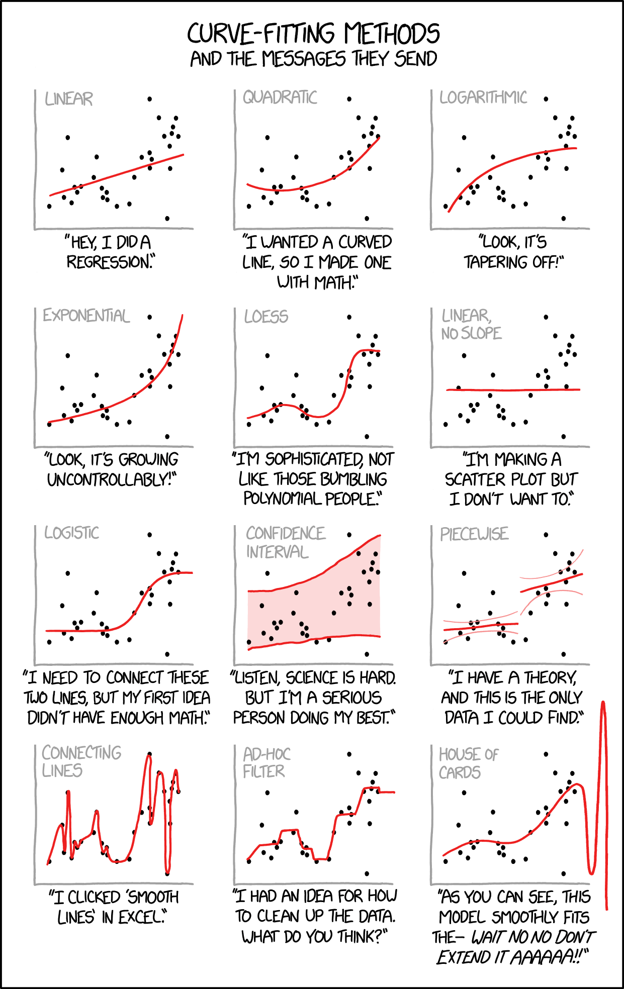
Check out the following xkcd comic. Which plot pokes fun at overfitting?

Part c

Check out some other goodies:

Exercise 7: Questioning R-squared

Zooming out, explain some limitations of relying on R-squared to measure the strength / usefulness of a model.

Exercise 8: Adjusted R-squared

We’ve observed that, unless a predictor is completely redundant with another predictor in our model, adding it to our model will increase R-squared. Even if that predictor is strongly multicollinear with another! Even if that predictor isn’t a good predictor!

Thus if we only look at R-squared we might get overly greedy. We can check our greedy impulses a few ways. We take a more in depth approach in STAT 253, but one quick alternative is reported right in our model summary() tables. Adjusted R-squared includes a penalty for incorporating more and more predictors. Mathematically, where \(n\) is the sample size and \(p\) is the number of non-intercept coefficients in our model:

\[ \text{Adjusted } R^2 = 1 - (1 - R^2) \left( \frac{n-1}{n-p-1} \right) \]

As we add more predictors into a model, R-squared increases, BUT the number of non-intercept coefficients \(p\) also increases. Thus unlike R-squared, Adjusted R-squared can decrease if the information that a predictor contributes to a model (reflected by R-squared) isn’t enough to offset the complexity it adds to that model (reflected by \(p\)). Consider two models:

example_mod_1 <- lm(bill_len ~ species, penguins)
example_mod_2 <- lm(bill_len ~ species + island, penguins)

Part a

Check out the summaries for the 2 example models and summarize your observations in this table:

Model	R-squared	Adj R-squared
bill_len ~ species	???	???
bill_len ~ species + island	???	???

Part b

In general, how does a model’s Adjusted R-squared compare to its R-squared? Is it greater, less than, or equal to the R-squared?

Part c

How did the R-squared change from example_mod_1 to example_mod_2? How did the Adjusted R-squared change?

Part d

Explain what it is about island that resulted in a decreased Adjusted R-squared. NOTE: it’s not necessarily the case that island is a bad predictor on its own!

Part e

Pulling this all together, which is the “better” of these 2 models?

Exercise 9: Reflection

Today we looked at some cautions surrounding indiscriminately adding variables to a model. Summarize key takeaways.

Exercise 10: Work on PP 4!!!

Solutions

Exercise 1: Modeling bill length by flipper length

model	predictors
`penguin_model_1`	`flipper_len`
`penguin_model_2`	`flipper_len_cm`
`penguin_model_3`	`flipper_len + flipper_len_cm`

Plots of the first two models are below:

ggplot(penguins, aes(y = bill_len, x = flipper_len)) + 
    geom_point() +
    geom_smooth(method = "lm", se = FALSE)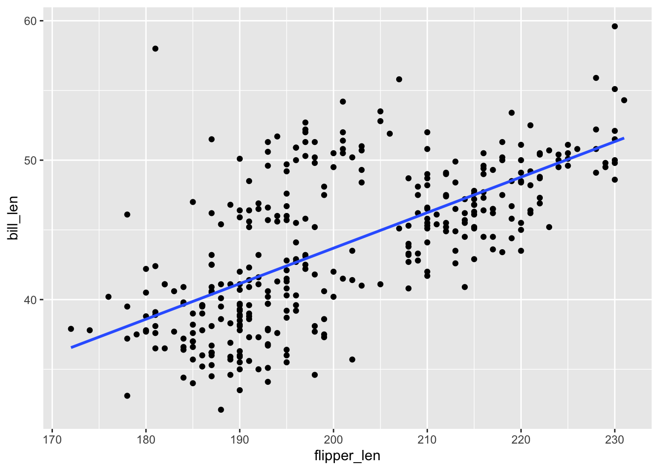


ggplot(penguins, aes(y = bill_len, x = flipper_len_cm)) + 
    geom_point() +
    geom_smooth(method = "lm", se = FALSE)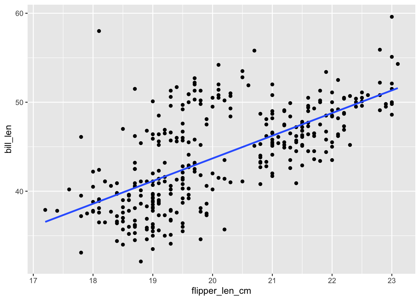

Your intuition–answers will vary
The R-squared values are all the same!

summary(penguin_model_1)$r.squared
## [1] 0.430574
summary(penguin_model_2)$r.squared
## [1] 0.430574
summary(penguin_model_3)$r.squared
## [1] 0.430574

The two variables are perfectly linearly correlated—they contain exactly the same information!

ggplot(penguins, aes(x = flipper_len, y = flipper_len_cm)) +
  geom_point()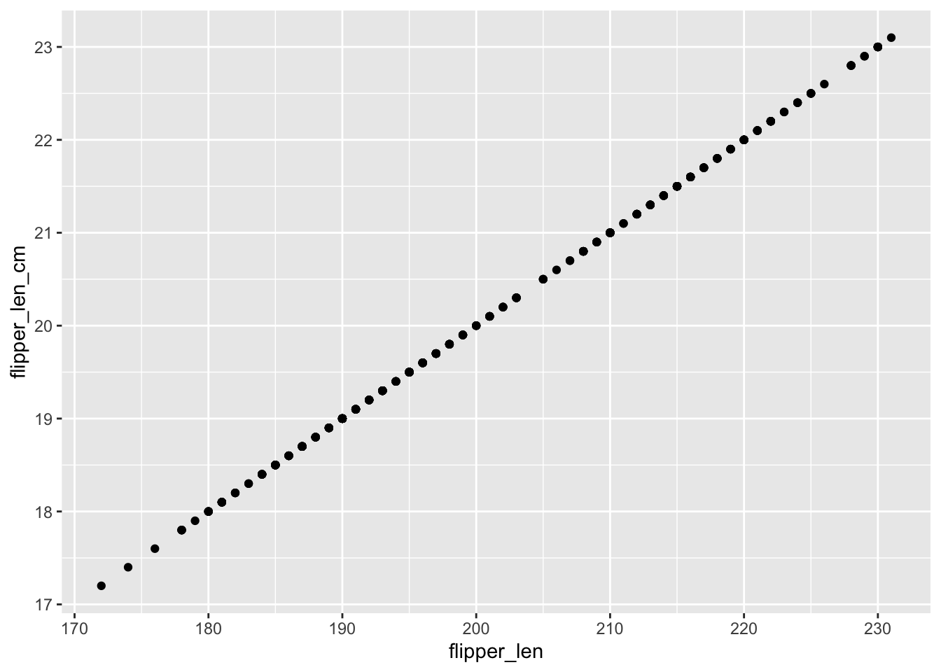

An NA means that the coefficient couldn’t be estimated. In penguin_model_3, the interpretation of the flipper_len_cm coefficient is the average change in bill length per centimeter change in flipper length, while holding flipper length in millimeters constant…this is impossible! We can’t hold flipper length in millimeters fixed while varying flipper length in centimeters—if one changes the other must. (In linear algebra terms, the matrix underlying our data is not of full rank.)

Exercise 2: Incorporating `body_mass`

model	predictors	R-squared
`penguin_model_1`	`flipper_len`	0.431
`penguin_model_4`	`body_mass`	0.354
`penguin_model_5`	`flipper_len + body_mass`	TBD (do NOT calculate)

flipper_len is a better predictor than body_mass because penguin_model_1 has an R-squared value of 0.431 vs 0.354 for penguin_model_4.
Intuition check–answers will vary
R-squared is for penguin_model_5 which is very slightly higher than that of penguin_model_1 and penguin_model_4.

summary(penguin_model_5)$r.squared
## [1] 0.4328544

d.flipper_len and body_mass are positively correlated and thus contain related information, but not completely redundant information. There’s some information in flipper length in explaining bill length that isn’t captured by body mass, and vice-versa.

ggplot(penguins, aes(x = flipper_len, y = body_mass)) +
  geom_point()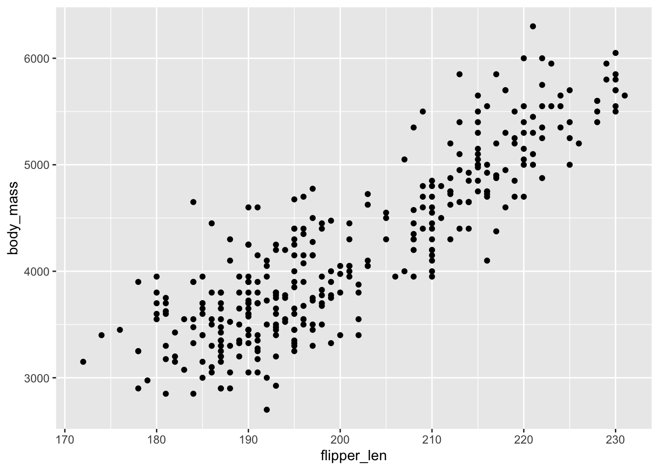

Exercise 3: Redundancy and Multicollinearity

model	predictors
`penguin_model_1`	`flipper_len`
`penguin_model_2`	`flipper_len_cm`
`penguin_model_3`	`flipper_len + flipper_len_cm`
`penguin_model_4`	`body_mass`
`penguin_model_5`	`flipper_len + body_mass`

penguin_model_3 had redundant predictors: flipper_len and flipper_len_cm
penguin_model_5 had multicollinear predictors: flipper_len and body_mass were related but not redundant
R-squared will stay the same if we add a redundant predictor to a model.
R-squared will increase by a small amount if we add a multicollinear predictor to a model.

Exercise 4: Considerations for strong models

# For illustration purposes only, take a sample of 10 penguins.
# We'll discuss this code later in the course!
set.seed(155)
penguins_small <- sample_n(penguins, size = 10) %>%
  mutate(flipper_len = jitter(flipper_len))
penguins_small %>% 
  ggplot(aes(y = bill_len, x = flipper_len)) + 
  geom_point()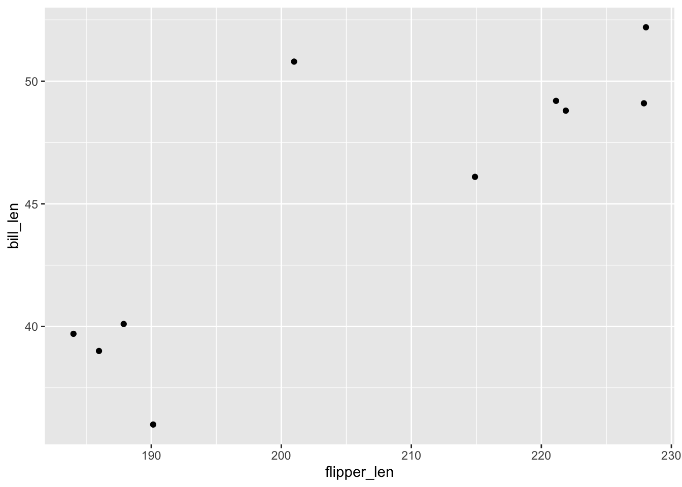

# A model with 1 predictor (flipper_len)
poly_mod_1 <- lm(bill_len ~ flipper_len, penguins_small)
# A model with 2 predictors (flipper_len and flipper_len^2)
poly_mod_2 <- lm(bill_len ~ poly(flipper_len, 2), penguins_small)
# A model with 9 predictors (flipper_len, flipper_len^2, ... on up to flipper_len^9)
poly_mod_9 <- lm(bill_len ~ poly(flipper_len, 9), penguins_small)

A gut check! Answers will vary
Based on R-squared: recall that R-squared is interpreted as the proportion of variation in the outcome that our model explains. It would seem that higher is better, so poly_mod_9 might seem to be the best. BUT we’ll see where this reasoning is flawed soon!

summary(poly_mod_1)$r.squared
## [1] 0.7341412
summary(poly_mod_2)$r.squared
## [1] 0.7630516
summary(poly_mod_9)$r.squared
## [1] 1

Based on the plots: Model 1! Definitely not Model 9

# A plot of model 1
ggplot(penguins_small, aes(y = bill_len, x = flipper_len)) + 
  geom_point() + 
  geom_smooth(method = "lm", se = FALSE)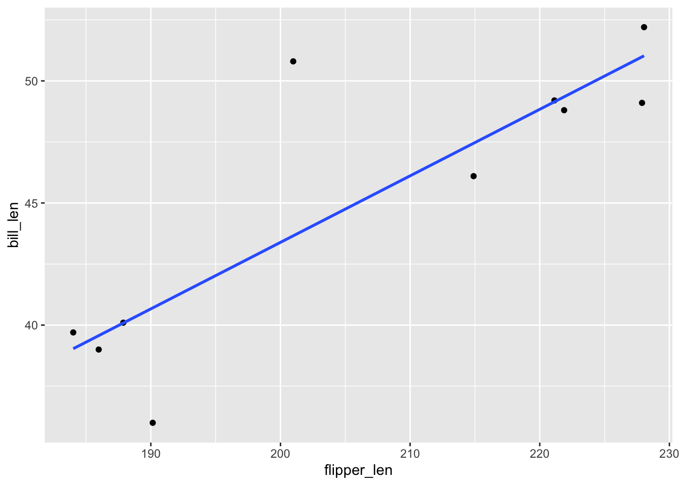

# A plot of model 2
ggplot(penguins_small, aes(y = bill_len, x = flipper_len)) + 
  geom_point() + 
  geom_smooth(method = "lm", formula = y ~ poly(x, 2), se = FALSE)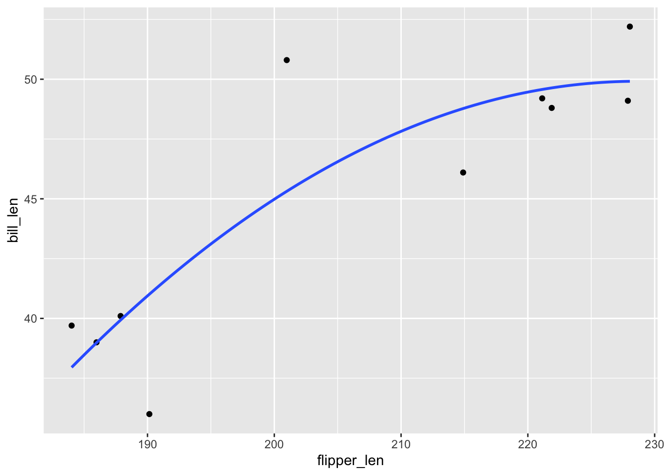

# A plot of model 9
ggplot(penguins_small, aes(y = bill_len, x = flipper_len)) + 
  geom_point() + 
  geom_smooth(method = "lm", formula = y ~ poly(x, 9), se = FALSE)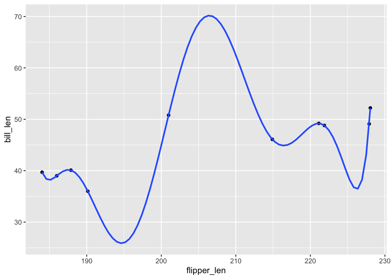

Exercise 5: Reflecting on these investigations

salmon, chocolate, samosas. Together? Yuck!
Regarding model 9:
- NOT easy to interpret.
- NO. It’s much more wiggly than the general trend.
- NOT WELL. It is too tailored to our data.

Exercise 6: Overfitting

The model picks up the tiny details of our original sample (red dots) at the cost of losing the more general trends of the relationship of interest (as demonstrated by the black dots).

penguins %>% 
  ggplot(aes(y = bill_len, x = flipper_len)) + 
  geom_point() +
  geom_smooth(method = "lm", formula = y ~ poly(x, 9), se = FALSE, data = penguins_small) +
  geom_point(data = penguins_small, color = "red", size = 3)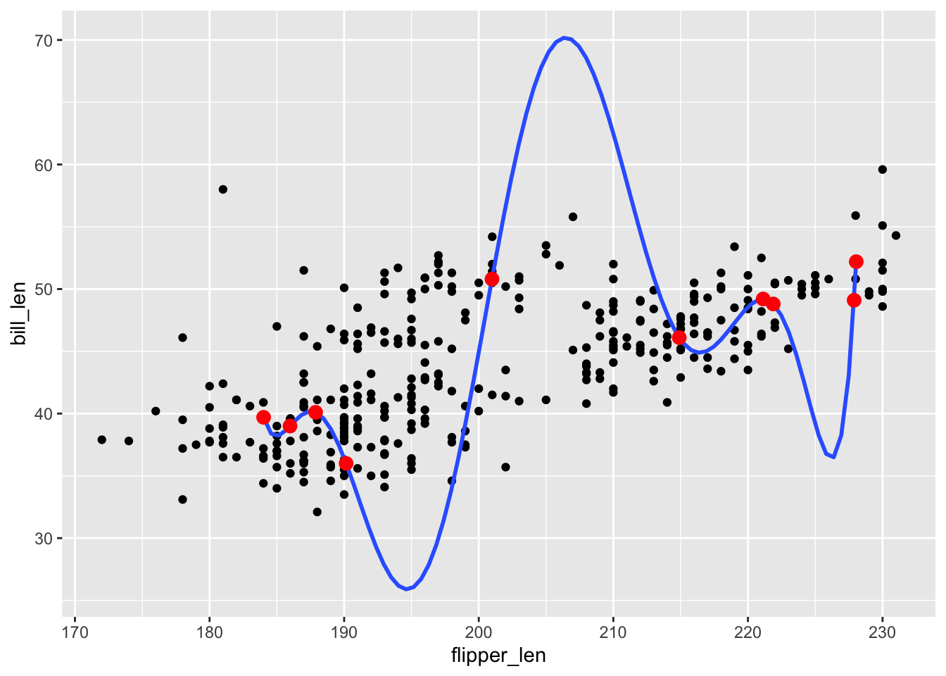

The bottom left plot pokes fun at overfitting.
funny.

Exercise 7: Questioning R-squared

It measures how well our model explains / predicts our sample data, not how well it explains / predicts the broader population. It also has the feature that any non-redundant predictor added to a model will increase the R-squared.

Exercise 8: Adjusted R-squared

Adjusted R-squared is less than the R-squared

Model	R-squared	Adj R-squared
bill_len ~ species	0.7078	0.7061
bill_len ~ species + island	0.7085	0.7051

example_mod_1 <- lm(bill_len ~ species, penguins)
example_mod_2 <- lm(bill_len ~ species + island, penguins)
summary(example_mod_1)
## 
## Call:
## lm(formula = bill_len ~ species, data = penguins)
## 
## Residuals:
##     Min      1Q  Median      3Q     Max 
## -7.9338 -2.2049  0.0086  2.0662 12.0951 
## 
## Coefficients:
##                  Estimate Std. Error t value Pr(>|t|)    
## (Intercept)       38.7914     0.2409  161.05   <2e-16 ***
## speciesChinstrap  10.0424     0.4323   23.23   <2e-16 ***
## speciesGentoo      8.7135     0.3595   24.24   <2e-16 ***
## ---
## Signif. codes:  0 '***' 0.001 '**' 0.01 '*' 0.05 '.' 0.1 ' ' 1
## 
## Residual standard error: 2.96 on 339 degrees of freedom
##   (2 observations deleted due to missingness)
## Multiple R-squared:  0.7078, Adjusted R-squared:  0.7061 
## F-statistic: 410.6 on 2 and 339 DF,  p-value: < 2.2e-16
summary(example_mod_2)
## 
## Call:
## lm(formula = bill_len ~ species + island, data = penguins)
## 
## Residuals:
##     Min      1Q  Median      3Q     Max 
## -7.9338 -2.2049 -0.0049  2.0951 12.0951 
## 
## Coefficients:
##                  Estimate Std. Error t value Pr(>|t|)    
## (Intercept)      38.97500    0.44697  87.198   <2e-16 ***
## speciesChinstrap 10.33204    0.53502  19.312   <2e-16 ***
## speciesGentoo     8.52988    0.52082  16.378   <2e-16 ***
## islandDream      -0.47321    0.59729  -0.792    0.429    
## islandTorgersen  -0.02402    0.61004  -0.039    0.969    
## ---
## Signif. codes:  0 '***' 0.001 '**' 0.01 '*' 0.05 '.' 0.1 ' ' 1
## 
## Residual standard error: 2.965 on 337 degrees of freedom
##   (2 observations deleted due to missingness)
## Multiple R-squared:  0.7085, Adjusted R-squared:  0.7051 
## F-statistic: 204.8 on 4 and 337 DF,  p-value: < 2.2e-16

Adjusted R-squared is lower than R-squared
From model 1 to 2, R-squared increased and Adjusted R-squared decreased.
island didn’t provide useful information about bill length beyond what was already provided by species.
example_mod_1. The improvement to R-squared by adding island to the model isn’t enough to offset the added complexity (Adj R-squared decreases).

Announcements etc

Warm-up

Exercises

Exercise 1: Modeling bill length by flipper length

Part a

Part b

Part c

Part d

Exercise 2: Incorporating body_mass

Part a

Part b

Part c

Part d

Exercise 3: Redundancy and Multicollinearity

Part a

Part b

Part c

Part d

Exercise 4: Considerations for strong models

Part a

Part b

Part c

Exercise 5: Reflecting on these investigations

Part a

Part b

Exercise 6: Overfitting

Part a

Part b

Part c

Exercise 7: Questioning R-squared

Exercise 8: Adjusted R-squared

Part a

Part b

Part c

Part d

Part e

Exercise 9: Reflection

Exercise 10: Work on PP 4!!!

Solutions

Exercise 1: Modeling bill length by flipper length

Exercise 2: Incorporating body_mass

Exercise 3: Redundancy and Multicollinearity

Exercise 4: Considerations for strong models

Exercise 5: Reflecting on these investigations

Exercise 6: Overfitting

Exercise 7: Questioning R-squared

Exercise 8: Adjusted R-squared

Exercise 2: Incorporating `body_mass`

Exercise 2: Incorporating `body_mass`