If you plan to use an extension, first check how many of the 3 available extensions you have left. These are tracked at the PP Extensions on Moodle.
If you’ve used 3 extensions, please remember that per course policy, future late PP / homework will not be accepted for credit. I recommend handing in whatever you have completed by the due date – it’s better to get partial credit than no credit.
Tuesday: Project final submission & reflection (pdf, qmd, reflection)
Finals week: Quiz 3
3:00-4:30pm section: Saturday, 12/13 from 1:30-3:30pm
1:20-2:50pm section: Tuesday, 12/16 from 1:30-3:30pm
Warm-up
p-value / testing cautionary tales: review from previous activity
fishing around for significance can lead to misleading conclusions. this is referred to as multiple testing.
the more things we test, the more likely something will appear to be “significant” just by chance (even if it’s not). this is a false positive or Type I error.
as with part b: fishing around for significance can lead to misleading conclusions
as with part a: don’t try to fit a hypothesis test into our narrative
Spotify example
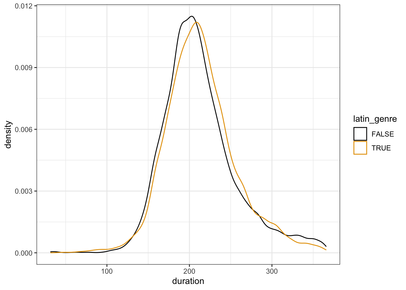
when sample size n is large, results might be statistically significant but not practically significant. that is, we might detect the existence of an effect, but the magnitude of the effect might be too small to be contextually meaningful.
why? standard errors decrease as n increases, and the smaller the s.e. the easier it is to detect coefficient deviations from 0.
# Load the dataspotify_big <-read.csv("https://ajohns24.github.io/data/spotify_example_big.csv") %>%select(track_artist, track_name, duration_ms, latin_genre) %>%mutate(duration = duration_ms /1000)nrow(spotify_big)## [1] 16216# Plot the relationshipspotify_big %>%ggplot(aes(x = duration, color = latin_genre)) +geom_density()
# Build the modelspotify_model_2 <-lm(duration ~ latin_genre, spotify_big)coef(summary(spotify_model_2))## Estimate Std. Error t value Pr(>|t|)## (Intercept) 212.673908 0.4165491 510.56143 0.00000000## latin_genreTRUE 1.555355 0.7435700 2.09174 0.03647731
The p-value debate
The p-value is very commonly misinterpreted and misused (usually unintentionally!). The following papers highlight a debate around the p-value: should we use them at all? and if so, what are best practices? I recommend skimming them outside of class!
Researchers report that people who regularly eat oatmeal for breakfast are significantly happier on a 0-10 scale (p-value = 0.015).
Interpret the p-value.
What statistical follow-up questions should you ask before taking this result seriously?
EXAMPLE 2: Never report a p-value alone
We should never report a p-value alone! It really means nothing on its own – we need the estimated magnitude of the effect and the error associated with this estimate. A few approaches for what to report / look for:
CI + p-value
estimate + standard error + p-value
estimate + CI + p-value
Let’s practice. Report what you learn about the relationship between the Price ($) of a home and its Age (years). NOTE: This data is from 2006!
homes <-read_csv("https://mac-stat.github.io/data/homes.csv")price_model <-lm(Price ~ Living.Area + Age, data = homes)summary(price_model)## ## Call:## lm(formula = Price ~ Living.Area + Age, data = homes)## ## Residuals:## Min 1Q Median 3Q Max ## -267300 -40485 -8491 27303 557613 ## ## Coefficients:## Estimate Std. Error t value Pr(>|t|) ## (Intercept) 22951.791 5536.960 4.145 3.56e-05 ***## Living.Area 111.277 2.713 41.019 < 2e-16 ***## Age -224.751 57.576 -3.904 9.84e-05 ***## ---## Signif. codes: 0 '***' 0.001 '**' 0.01 '*' 0.05 '.' 0.1 ' ' 1## ## Residual standard error: 68820 on 1725 degrees of freedom## Multiple R-squared: 0.5118, Adjusted R-squared: 0.5112 ## F-statistic: 904.2 on 2 and 1725 DF, p-value: < 2.2e-16
EXAMPLE 3 (OPTIONAL): Power
Statistical power is the probability of rejecting the null hypothesis when the alternative hypothesis is true (a “true positive”). For example, in the tests we’ve been doing, statistical power is the probability of detecting a relationship when there truly is a relationship.
Check out this interactive visualization of the factors that influence statistical power:
Under “Settings”, next to the “Solve for?” text, click “Power”. You will vary the 3 different parameters (significance level, sample size, and effect size) one at a time to understand how these factors affect power. Some (OPTIONAL) context behind this interactive visualization:
Visualization is based on a one sample Z-test:
This is a test for whether the true population mean equals a particular value. (e.g., true mean = 30)
The effect size slider is measured with a metric called Cohen’s d:
Cohen’s d = magnitude of effect/standard deviation of response variable
Here: how far is the true mean from the null value in units of SD?
e.g., If the null value is 30, true mean is 40, and the true population SD of the quantity is 5, the Cohen’s d effect size is (40-30)/5 = 2.
What is your intuition about how changing the significance level will change power? Check your intuition with the visualization and explain why this happens.
Repeat Part a for the sample size.
Repeat Part a for the effect size.
Project time
Discuss Project Milestone 2 feedback.
Discuss what needs to be done for the final project submission.
Everyone should have a hand in every aspect of the project (eg: planning the analysis, writing code, writing up the report, etc). But it would be helpful to divvy up who will write the first draft of each section in the report.
Everyone is expected to review and provide feedback on the entire report + qmd code file.
Pro tip: use the provided rubric in your editing and feedback process!
Solutions
EXAMPLE 1: Never trust a p-value alone
There’s only a 1.5% chance that the researchers would’ve observed such a difference in happiness among their sample of people who do and don’t eat oatmeal IF in fact happiness levels truly don’t differ between these 2 groups.
.
What’s the magnitude of observed difference? 2 points? 0.001 points?
Relatedly, were there a lot of people in the sample? Could the results be statistically but not practically significant?
Did they control for potential confounders (e.g. age, income, etc)?
EXAMPLE 2: Never report a p-value alone
homes <-read_csv("https://mac-stat.github.io/data/homes.csv")price_model <-lm(Price ~ Living.Area + Age, data = homes)summary(price_model)## ## Call:## lm(formula = Price ~ Living.Area + Age, data = homes)## ## Residuals:## Min 1Q Median 3Q Max ## -267300 -40485 -8491 27303 557613 ## ## Coefficients:## Estimate Std. Error t value Pr(>|t|) ## (Intercept) 22951.791 5536.960 4.145 3.56e-05 ***## Living.Area 111.277 2.713 41.019 < 2e-16 ***## Age -224.751 57.576 -3.904 9.84e-05 ***## ---## Signif. codes: 0 '***' 0.001 '**' 0.01 '*' 0.05 '.' 0.1 ' ' 1## ## Residual standard error: 68820 on 1725 degrees of freedom## Multiple R-squared: 0.5118, Adjusted R-squared: 0.5112 ## F-statistic: 904.2 on 2 and 1725 DF, p-value: < 2.2e-16
We have evidence of a significant association between home price and age when controlling for size (p-value = 9.84e-05). Specifically, when controlling for size, we’re 95% confident that the expected home price decreases by somewhere between $110 and $340 for each 1-year increase in age.
# CI for Age coef-224.751-2*57.576## [1] -339.903-224.751+2*57.576## [1] -109.599