library(tidyverse)
elections <- read_csv("https://ajohns24.github.io/data/election_2024.csv") %>%
  mutate(repub_24 = round(100*per_gop_2024, 2),
         repub_20 = round(100*per_gop_2020, 2),
         repub_16 = round(100*per_gop_2016, 2),
         repub_12 = round(100*per_gop_2012, 2)) %>%
  select(state_name, state_abbr, county_name, county_fips, repub_24, repub_20, repub_16, repub_12)

head(elections)

population_model <- lm(repub_24 ~ repub_12, data = elections)
summary(population_model)16 Sampling distributions, CLT, & Bootstrapping
Announcements etc
SETTLING IN
Find the qmd here: “16-sampling-dist-clt-bootstrap-notes.qmd”.
Install the
mosaicpackage from the Packages tab.- If you get an error: Re-install the
tidyversepackage from the Packages tab.
- If you get an error: Re-install the
WRAPPING UP
Upcoming due dates:
- This week
- Thursday = Project Milestone 1 Use the template and directions on Moodle!
- Next week
- Tuesday
- Quiz 2 revisions (at the start of class)
Follow the directions on Moodle! If you follow directions, you can get up to 50% of points back. If you don’t follow directions, you can get up to 33% of points back. - CP 14
- Quiz 2 revisions (at the start of class)
- Thursday
- PP 6
- Tuesday
- Related but unrelated: MSCS events calendar
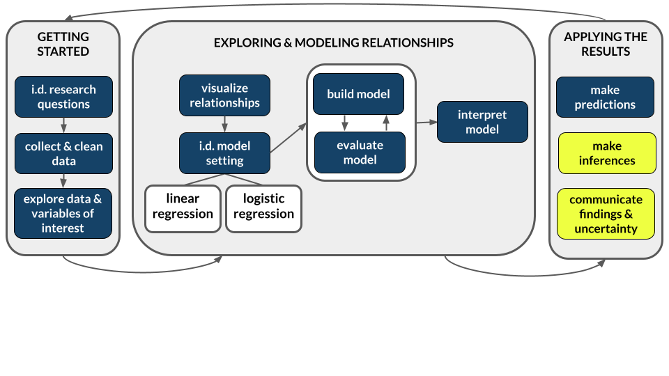
Learning goals
Let \(\beta\) be some population parameter and \(\hat{\beta}\) be a sample estimate of \(\beta\). Our goals for the day are to:
- use simulation to solidify our understanding of sampling distributions and standard errors
- explore and compare two approaches to approximating the sampling distribution of \(\hat{\beta}\):
- Central Limit Theorem (CLT)
- bootstrapping
- explore the impact of sample size on sampling distributions and standard errors
Additional resources
References
Let \(\beta\) be some population parameter that we want to estimate with sample statistic \(\hat{\beta}\).
Sampling distributions help us understand the potential error in our sample estimate \(\hat{\beta}\)
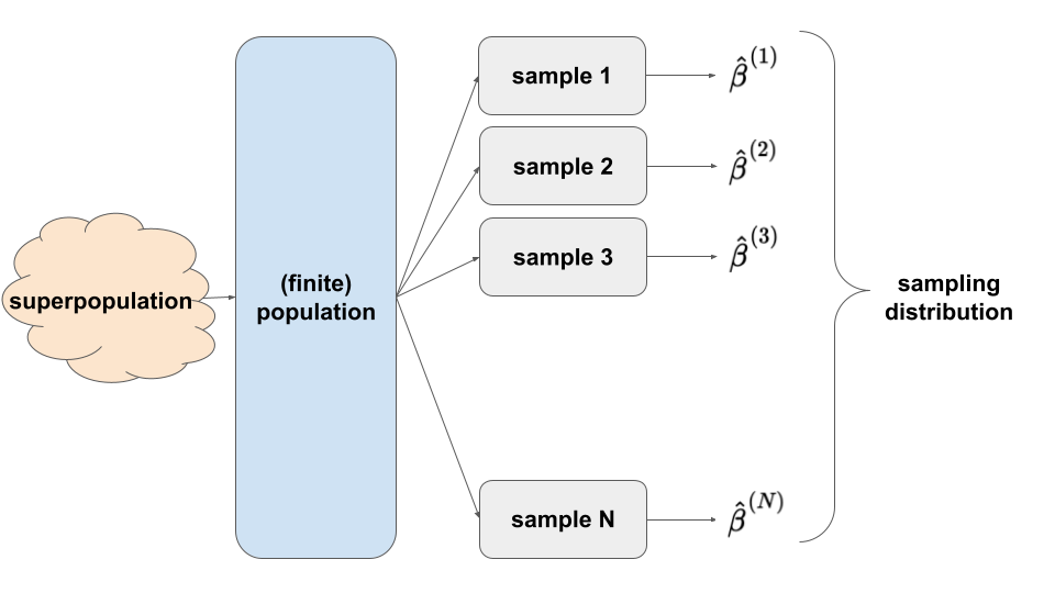
The sampling distribution of \(\hat{\beta}\) is a collection of all possible estimates we could observe based on all possible samples of the same size n from the population. A sampling distribution captures the degree to which a sample estimate can vary from the actual population value, hence the potential error in a sample estimate.
The snag: we can’t know exactly how wrong our estimate is.
In practice, we only take ONE sample, thus can’t actually observe the sampling distribution.
Though we can’t observe the sampling distribution, we can APPROXIMATE it using the Central Limit Theorem.
So long as certain conditions are met (e.g. our sample size n is “big enough”), then the sampling distribution of \(\hat{\beta}\) is Normally distributed around the actual population value \(\beta\) with some standard error:
\[\hat{\beta} \sim N(\beta, \text{(standard error)}^2)\]
The standard error, i.e. standard deviation among all possible estimates \(\hat{\beta}\), measures the typical estimation error (i.e. the typical difference between \(\hat{\beta}\) and \(\beta\)).
Warm-Up
WHERE ARE WE?
Sample vs population
- We have data on a sample that we want to use to learn about the broader population.
- Eg: We can use a sample statistic \(\hat{\beta}\) to estimate population parameter \(\beta\).
Sampling variability
Ours is one of many samples we might have gotten from the population.Sampling error
Since our sample isn’t the population itself, there’s error in using our data to estimate features of the population.Ethics
We must understand and report the potential error in our estimate.Sampling distributions
- A sampling distribution describes the different sample estimates we might get, i.e. how \(\hat{\beta}\) might vary from sample to sample.
- Hence they provide a sense of the potential error in our sample estimate.
SAMPLING DISTRIBUTION
ELECTION EXAMPLE
Recall our election example where Y is the Republican candidate’s (Trump’s) 2024 county-level vote percentage, and X is the Republican candidate’s (Mitt Romney’s) 2012 vote percentage. Based on data from the entire population of U.S. counties (except Alaska), we can obtain the “true” population model of Y vs X:
\[ E[Y|X] = \beta_0 + \beta_1 X = 9.699 + 0.957 X \]
EXAMPLE 1: Simulating the sampling distribution (500 samples of size 50)
In the previous activity, each student took 1 sample of 50 counties without replacement:
# Run this chunk a few times to explore the different sample models you get
elections %>%
  sample_n(size = 50, replace = FALSE)
We can also take a sample and then use it to estimate the population model:
# Run this chunk a few times to explore the different sample models you get
elections %>%
  sample_n(size = 50, replace = FALSE) %>%
  with(lm(repub_24 ~ repub_12))
In the previous class, we obtained a collection of sample estimates by having each student take 1 sample and share their results. BUT we each have the power to simulate this process on our own:
# Set the random number seed
set.seed(155)

# Obtain  *500* separate samples of *50 counties each*
# Store the sample models from each
election_models_50 <- mosaic::do(500)*(
  elections %>%
    sample_n(size = 50, replace = FALSE) %>%
    with(lm(repub_24 ~ repub_12))
)
# Check it out
head(election_models_50)
dim(election_models_50)Questions
What’s the point of the
do()function?!? If you’ve taken any COMP classes, what process do you thinkdo()is a shortcut for?What is stored in the
Intercept,repub_12, andr.squaredcolumns of the results?
EXAMPLE 2: Checking out the sampling distribution
Recall the actual population model:
\[ E[Y|X] = \beta_0 + \beta_1 X = 9.699 + 0.957 X \]
# Plot the 500 sample plots (gray) relative to the actual population model (red):
elections %>%
  ggplot(aes(x = repub_12, y = repub_24)) +
  geom_smooth(method = "lm", se = FALSE) +
  geom_abline(data = election_models_50,
              aes(intercept = Intercept, slope = repub_12),
              color = "gray", size = 0.25) +
  geom_smooth(method = "lm", color = "red", se = FALSE)
Check out the (approximate) sampling distribution of the estimated slope coefficient \(\hat{\beta}_1\), relative to the actual slope coefficient \(\beta_1 = 0.957\) (red):
# Approximate sampling distribution of the slope estimate
election_models_50 %>%
  ggplot(aes(x = repub_12)) +
  geom_density() +
  geom_vline(xintercept = 0.957, color = "red")
Recall that the standard deviation of the estimated sample slope coefficients \(\hat{\beta}_1\) is referred to as the standard error of \(\hat{\beta}_1\):
\[ s.e.(\hat{\beta}_1) \]
It measures the typical distance of a sample slope from the actual population slope \(\beta_1\), i.e. the standard error. In our simulation, the standard error of the sample slope coefficients is 0.076:
# Approximate standard error of the slope estimate
election_models_50 %>%
  summarize(sd(repub_12))
Reflection: Interpret the standard error.
BUT! What actually happens in practice?
We only take 1 sample of, say, 50 counties. (We don’t go out and take 500 different samples of 50 counties.)
- Thus we don’t have access to the sampling distribution…
- Thus we don’t actually know the standard error of the sample estimates…
- Thus we need to approximate the sampling distribution / standard error using our 1 sample.
We’ll take 2 different approaches:
- Central Limit Theorem (formula-based approach)
- Bootstrapping (simulation-based approach)
EXAMPLE 3: 1 sample of fish
Rivers contain small concentrations of mercury which can accumulate in fish. Scientists studied this phenomenon among largemouth bass in the Wacamaw and Lumber rivers of North Carolina. One goal was to explore the relationship of a fish’s mercury concentration (Concen) in parts per million (ppm) with its size, as measured by Length (cm):
\[ E(Concen | Length) = \beta_0 + \beta_1 Length \]
To estimate this relationship, they caught and evaluated 171 fish:
# Load the data
fish <- read_csv("https://Mac-STAT.github.io/data/Mercury.csv")Superpopulation: The true underlying process that governs the relationship between mercury concentration and length of fish, for every fish that has ever existed and ever will exist in these two rivers!
Finite Population: At the time the data was collected, the true relationship between mercury concentration and length of fish, for all fish in the two rivers at that time.
Sample: Our sample of 171 fish!!!
EXAMPLE 4: Approximate the sampling distribution via the CLT
# Plot the SAMPLE relationship along with the SAMPLE model estimate
fish %>%
  ggplot(aes(y = Concen, x = Length)) +
  geom_point() +
  geom_smooth(method = "lm", se = FALSE)
# Obtain the SAMPLE model
fish_model <- lm(Concen ~ Length, data = fish)
coef(summary(fish_model))What’s \(\beta_1\), the actual population
Lengthcoefficient?What’s \(\hat{\beta}_1\), the sample estimate of the population
Lengthcoefficient?The table above reports an approximated standard error of \(\hat{\beta}_1\). This was calculated via some formula \(c / \sqrt{n}\) (using mathematical theory, not simulation). What is it?
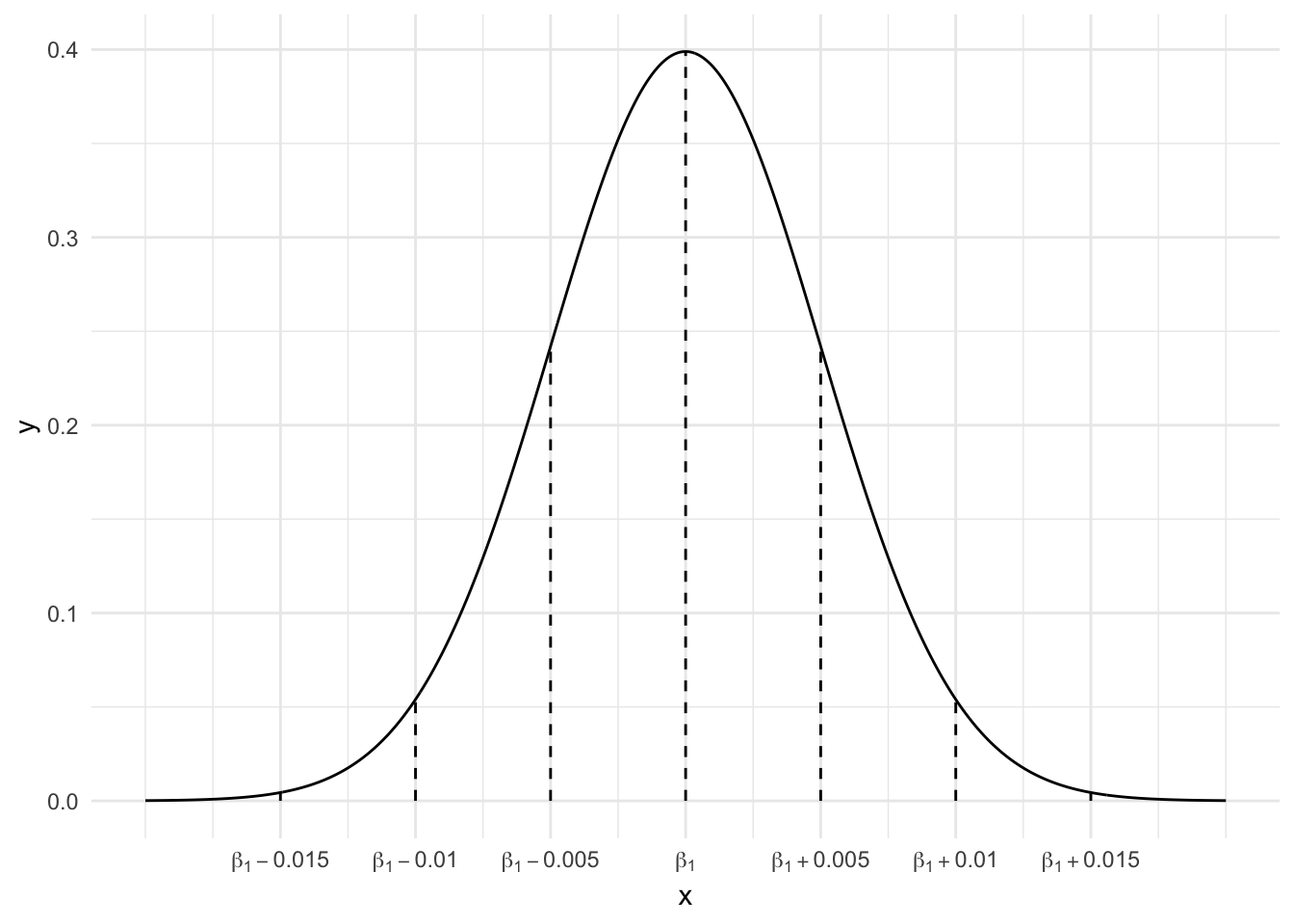
State the CLT in this setting, and sketch it (on paper). Mark it according to the “68-95-99.7 Rule”
Where does our estimate \(\hat{\beta}_1\) fall on this picture (e.g. is it above / below / close to / far from \(\beta_1\)?)? Or is this a trick question?
Approximate the sampling distribution via Bootstrapping
Recall the sampling distribution:
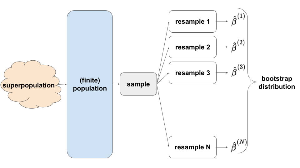
Whereas the CLT approximates the sampling distribution via theoretical assumptions, the bootstrapping technique approximates the sampling distribution via simulation. In practice, we can’t simulate the sampling distribution by repeatedly taking samples (as in the election example) – we only take 1 sample of size n!! But we can REsample our sample:
- we sample our sample WITH replacement (you’ll explore why below)
- each REsample is of size n, the same size as the original sample (so that we can assess the potential error associated with samples the same size as ours)
This helps us approximate the shape of the sampling distribution and the standard error of our estimate:
The saying “to pull oneself up by the bootstraps” is often attributed to Rudolf Erich Raspe’s 1781 The Surprising Adventures of Baron Munchausen in which the character pulls himself out of a swamp by his hair (not bootstraps). In short, it means to get something from nothing, through your own effort:

In this spirit, statistical bootstrapping doesn’t make any probability model assumptions. It uses only the information from our one sample to approximate standard errors.
Approximating the sampling distribution: CLT vs Bootstrapping
- CLT
- The quality of this approximation hinges upon the validity of the Central Limit Theorem which hinges upon the validity of the theoretical model assumptions, as well as a “large enough” sample size n.
- The CLT uses theoretical formulas for the standard error estimates, thus can feel a little mysterious without a solid foundation in probability theory.
- BUT: When the theory is “valid”, nothing beats a CLT approximation!!!
- Bootstrapping
- The statistical theory behind bootstrapping is quite complicated, and there are certain obscure cases (none that we will encounter in STAT 155) where the assumptions underlying bootstrapping fail to hold.
- It cannot and should not replace the CLT. BUT, it but gives us some nice intuition behind the idea of resampling, which is fundamental for hypothesis testing (which we’ll get to shortly!).
Exercises
Goals:
- Learn how to implement the bootstrapping technique.
- Use bootstrapping to explore the impact of sample size on standard errors, and the sampling distribution more generally.
Exercise 1: Why “resampling” (replace = TRUE)?
Recall that in bootstrapping, we REsample our sample – we sample it without replacement. Let’s wrap our minds around this idea using a small example of just the first 4 fish in our data:
small_sample <- fish %>%
select(Concen, Length) %>%
head(4)
small_sampleThis sample produces an estimated Length coefficient of 0.06532:
lm(Concen ~ Length, data = small_sample)Part a
The chunk below samples 4 fish from the small_sample without replacement (replace = FALSE). Run it several times, then discuss:
- What do you observe about the samples themselves?
- If we used each one of these samples to estimate the model of
ConcenbyLength, what do you anticipate will happen?
sample_n(small_sample, size = 4, replace = FALSE)Part b
Test your intuition. The chunk below samples 4 fish from the small_sample without replacement (replace = FALSE), then uses it to estimate the model of Concen by Length. Run it several times, then discuss:
- What do you observe about the sample models?
- What’s the problem with this?
sample_n(small_sample, size = 4, replace = FALSE) %>%
with(lm(Concen ~ Length))Part c
Sampling our sample without replacement merely returns our original sample, thus does NOT give us any sense of sampling variability! Instead, REsample 4 fish from our small_sample with replacement. Run it several times. What do you notice about the samples themselves?
sample_n(small_sample, size = 4, replace = TRUE)Similarly, what do you notice about the sample models built from the REsamples?
sample_n(small_sample, size = 4, replace = TRUE) %>%
with(lm(Concen ~ Length))
Reflect: Resampling
REsampling our sample provides insight into sampling variability, hence potential error in our sample estimates. Each REsample might include some original sample subjects several times, and others not at all. But this is a good thing!
- Observing a subject multiple times in a REsample mimics the idea that there are several separate but similar subjects in the population!
- Sampling with replacement ensures that our resampled observations are independent, which we need in order for bootstrapping to “work”!
Exercise 2: Run a bootstrap simulation
We’ll obtain a bootstrapping distribution of \(\hat{\beta}_1\) by taking many (500, in this case) different samples of every fish in our dataset (171 of them) and exploring the degree to which \(\hat{\beta}_1\) varies from sample to sample.
Edit the code below to obtain a bootstrapping distribution.
# Set the seed so that we all get the same results
set.seed(155)
# Store the sample models
sample_models_171 <- mosaic::do(___)*(
fish %>%
___(size = ___, replace = ___) %>%
with(___(Concen ~ Length))
)
# Check out the first 6 results
# Make sure that your first Intercept estimate is -1.1802375
head(sample_models_171)
Exercise 3: Bootstrap vs CLT sampling distribution
Check out the resulting 500 bootstrapped sample models. The red line represents the model estimate calculated from our original sample of 171 fish (not the population model, which we don’t know!):
fish %>%
ggplot(aes(x = Length, y = Concen)) +
geom_smooth(method = "lm", se = FALSE) +
geom_abline(data = sample_models_171,
aes(intercept = Intercept, slope = Length),
color = "gray", size = 0.25) +
geom_smooth(method = "lm", color = "red", se = FALSE)Let’s focus on the slopes of these 500 sample models.
Part a
A plot of our 500 bootstrap slopes approximates the actual sampling distribution:
sample_models_171 %>%
ggplot(aes(x = Length)) +
geom_density()Describe the sampling distribution:
What’s its general shape?
Where is it roughly centered? Is this value the “true” population slope \(\beta_1\) or our sample slope estimate \(\hat{\beta}_1\)?
Roughly what’s its spread, i.e. what’s the range of estimates you observed?
Part b
For a more rigorous assessment of the spread among the bootstrap slopes, calculate their standard deviation. This provides a bootstrap approximation of the standard error of the slope estimates:
sample_models_171 %>%
___(sd(Length))Part c
Recall that the bootstrap and CLT both aim to approximate features of the sampling distribution of sample slope \(\hat{\beta}_1\). In the warm-up, we noted that the CLT assumed that the sample estimates are Normally distributed around the “true” population slope \(\beta_1\) with an estimated standard error of 0.005. In contrast, since they’re obtained from resampling the original sample of 171 fish, the bootstrapping results are distributed around the original sample slope. However, and importantly:
Is the shape of the bootstrapping results in Part a consistent with the CLT assumptions of Normality?
Is the spread / standard error of the bootstrapping results in Part b consistent with the CLT approximation of the standard error (0.005)?
Exercise 4: Increasing sample size – intuition
Now that we trust bootstrapping simulations to provide reasonable insight into sampling distributions, let’s use them to explore the impact of sample size on the quality of our sample estimates. Recall our different (bootstrap) sample estimates when we started with a sample of 171 fish:
# All bootstrap sample models
fish %>%
ggplot(aes(x = Length, y = Concen)) +
geom_smooth(method = "lm", se = FALSE) +
geom_abline(data = sample_models_171,
aes(intercept = Intercept, slope = Length),
color = "gray", size = 0.25)# Slopes of all bootstrap sample models
sample_models_171 %>%
ggplot(aes(x = Length)) +
geom_density()Suppose that instead of starting with n = 171 fish, we only had a sample of n = 50 or n = 20 fish! What impact do you anticipate this having on our sample estimates:
If we had a smaller sample, how would it impact the sample model lines (top plot): Do you expect there to be more or less variability among the sample model lines?
If we had a smaller sample, how would it impact the sampling distribution of the sample slopes (bottom plot):
- Around what value to you expect it be centered?
- What general shape do you expect it to have?
- Do you expect it to be narrower (with smaller standard error) or wider (with larger standard error)?
Exercise 5: 500 samples of size n
Let’s decrease the sample size in our simulation. First, take 500 REsamples from fish, but this time make each resample just 50 fish. Then build a sample model from each sample:
set.seed(155)
sample_models_50 <- mosaic::___(500)*(
fish %>%
___(size = ___, replace = TRUE) %>%
___(___(Concen ~ Length))
)
# Check it out
# Make sure that your first Intercept estimate is -1.1602313
head(sample_models_50)Similarly, take 500 REsamples of size 20 from fish, then build a sample model from each sample:
set.seed(155)
sample_models_20 <- mosaic::___(500)*(
fish %>%
___(size = ___, replace = TRUE) %>%
___(___(Concen ~ Length))
)
# Check it out
# Make sure that your first Intercept estimate is -2.3961270
head(sample_models_20)
Exercise 6: Impact of sample size (part I)
Use the 3 plots below to compare and contrast the 500 sets of sample models when using samples of size 20, 50, and 171. What happens as we increase sample size?! Was this what you expected?
# 500 sample models using samples of size 20
fish %>%
ggplot(aes(x = Length, y = Concen)) +
geom_smooth(method = "lm", se = FALSE) +
geom_abline(data = sample_models_20,
aes(intercept = Intercept, slope = Length),
color = "gray", size = 0.25) +
lims(x = c(25, 65), y = c(-1, 5))# 500 sample models using samples of size 50
fish %>%
ggplot(aes(x = Length, y = Concen)) +
geom_smooth(method = "lm", se = FALSE) +
geom_abline(data = sample_models_50,
aes(intercept = Intercept, slope = Length),
color = "gray", size = 0.25) +
lims(x = c(25, 65), y = c(-1, 5))# 500 sample models using samples of size 171
fish %>%
ggplot(aes(x = Length, y = Concen)) +
geom_smooth(method = "lm", se = FALSE) +
geom_abline(data = sample_models_171,
aes(intercept = Intercept, slope = Length),
color = "gray", size = 0.25) +
lims(x = c(25, 65), y = c(-1, 5))
Exercise 7: Impact of sample size (part II)
Using the 3 plots below, let’s focus on just the sampling distributions of our 500 slope estimates \(\hat{\beta}_1\), i.e. the slopes of the lines in the above plots. How do the shapes, centers, and spreads of these sampling distributions compare? Was this what you expected?
# 500 sample slopes using samples of size 20
sample_models_20 %>%
ggplot(aes(x = Length)) +
geom_density() +
lims(x = c(-0.01, 0.13), y = c(0, 70))# 500 sample slopes using samples of size 50
sample_models_50 %>%
ggplot(aes(x = Length)) +
geom_density() +
lims(x = c(-0.01, 0.13), y = c(0, 70))# 500 sample slopes using samples of size 171
sample_models_171 %>%
ggplot(aes(x = Length)) +
geom_density() +
lims(x = c(-0.01, 0.13), y = c(0, 70))
Exercise 8: Properties of sampling distributions
In light of your observations, complete the following statements about the sampling distribution of the sample slope.
For all sample sizes, the shape of the sampling distribution is roughly ___ and is roughly centered around the same location. (NUANCE: Here the estimates vary around the original sample slope since we’re resampling from the sample. But in theory, different samples from the population will produce sample slopes that vary around the population slope!)
As sample size increases:
The average sample slope estimate INCREASES / DECREASES / IS FAIRLY STABLE.
The standard error of the sample slopes INCREASES / DECREASES / IS FAIRLY STABLE.Thus, as sample size increases, estimates of the slope become MORE RELIABLE / LESS RELIABLE.
Just for fun
Want more intuition into sampling distributions and the CLT? Watch this video explanation using bunnies and dragons: https://www.youtube.com/watch?v=jvoxEYmQHNM
Solutions
library(tidyverse)
elections <- read_csv("https://ajohns24.github.io/data/election_2024.csv") %>%
mutate(repub_24 = round(100*per_gop_2024, 2),
repub_20 = round(100*per_gop_2020, 2),
repub_16 = round(100*per_gop_2016, 2),
repub_12 = round(100*per_gop_2012, 2)) %>%
select(state_name, state_abbr, county_name, county_fips, repub_24, repub_20, repub_16, repub_12)
head(elections)
## # A tibble: 6 × 8
## state_name state_abbr county_name county_fips repub_24 repub_20 repub_16
## <chr> <chr> <chr> <dbl> <dbl> <dbl> <dbl>
## 1 Alabama AL Autauga County 1001 72.7 71.4 73.4
## 2 Alabama AL Baldwin County 1003 78.6 76.2 77.4
## 3 Alabama AL Barbour County 1005 57.0 53.4 52.3
## 4 Alabama AL Bibb County 1007 81.9 78.4 77.0
## 5 Alabama AL Blount County 1009 90.2 89.6 89.8
## 6 Alabama AL Bullock County 1011 26.8 24.8 24.2
## # ℹ 1 more variable: repub_12 <dbl>
population_model <- lm(repub_24 ~ repub_12, data = elections)
summary(population_model)
##
## Call:
## lm(formula = repub_24 ~ repub_12, data = elections)
##
## Residuals:
## Min 1Q Median 3Q Max
## -25.902 -4.172 0.352 4.462 35.645
##
## Coefficients:
## Estimate Std. Error t value Pr(>|t|)
## (Intercept) 9.699197 0.522156 18.57 <2e-16 ***
## repub_12 0.957318 0.008472 113.00 <2e-16 ***
## ---
## Signif. codes: 0 '***' 0.001 '**' 0.01 '*' 0.05 '.' 0.1 ' ' 1
##
## Residual standard error: 6.926 on 3098 degrees of freedom
## (69 observations deleted due to missingness)
## Multiple R-squared: 0.8048, Adjusted R-squared: 0.8047
## F-statistic: 1.277e+04 on 1 and 3098 DF, p-value: < 2.2e-16
EXAMPLE 1: Simulating the sampling distribution (500 samples of size 50)
# Run this chunk a few times to explore the different sample models you get
elections %>%
sample_n(size = 50, replace = FALSE)
## # A tibble: 50 × 8
## state_name state_abbr county_name county_fips repub_24 repub_20 repub_16
## <chr> <chr> <chr> <dbl> <dbl> <dbl> <dbl>
## 1 Oklahoma OK Oklahoma Co… 40109 49.7 49.2 51.7
## 2 Nebraska NE Wayne County 31179 73.9 72.4 71.5
## 3 Iowa IA Washington … 19183 61.6 59.2 57
## 4 Ohio OH Pickaway Co… 39129 73.8 72.8 69.2
## 5 Ohio OH Athens Coun… 39009 44.2 41.7 38.7
## 6 Indiana IN Greene Coun… 18055 76.1 75.1 74.7
## 7 Wisconsin WI Waukesha Co… 55133 59.2 59.6 61.1
## 8 South Carolina SC Greenwood C… 45047 63.8 60.7 59.0
## 9 Colorado CO Yuma County 8125 81.6 82.4 80.5
## 10 Ohio OH Adams County 39001 82.6 81.3 76.3
## # ℹ 40 more rows
## # ℹ 1 more variable: repub_12 <dbl># Run this chunk a few times to explore the different sample models you get
elections %>%
sample_n(size = 50, replace = FALSE) %>%
with(lm(repub_24 ~ repub_12))
##
## Call:
## lm(formula = repub_24 ~ repub_12)
##
## Coefficients:
## (Intercept) repub_12
## 19.9168 0.8149# Set the random number seed
set.seed(155)
# Obtain *500* separate samples of *50 counties each*
# Store the sample models from each
election_models_50 <- mosaic::do(500)*(
elections %>%
sample_n(size = 50, replace = FALSE) %>%
with(lm(repub_24 ~ repub_12))
)
# Check it out
head(election_models_50)
## Intercept repub_12 sigma r.squared F numdf dendf .row .index
## 1 14.909924 0.8776792 6.240864 0.8074511 201.28738 1 48 1 1
## 2 12.071268 0.9298640 7.023377 0.7649355 146.43686 1 45 1 2
## 3 15.384365 0.8565752 9.049565 0.6491243 86.95057 1 47 1 3
## 4 11.727596 0.9217806 6.555849 0.8487826 252.58476 1 45 1 4
## 5 10.286748 0.9433663 7.039844 0.8050256 194.05728 1 47 1 5
## 6 4.018903 1.0429749 5.721746 0.8459846 252.67135 1 46 1 6
dim(election_models_50)
## [1] 500 9Questions
do()repeats the code within the parentheses as many times as you tell it. do()` is a shortcut for a for loop.- This process produces 500 sample model estimates, built from different samples of size 50. The
Interceptandrepub_12columns contain the coefficient estimates for each of these 500 models. Ther.squaredcolumn contains the R-squared values for these 500 models.
EXAMPLE 2: Checking out the sampling distribution
# Plot the 500 sample plots (gray) relative to the actual population model (red):
elections %>%
ggplot(aes(x = repub_12, y = repub_24)) +
geom_smooth(method = "lm", se = FALSE) +
geom_abline(data = election_models_50,
aes(intercept = Intercept, slope = repub_12),
color = "gray", size = 0.25) +
geom_smooth(method = "lm", color = "red", se = FALSE)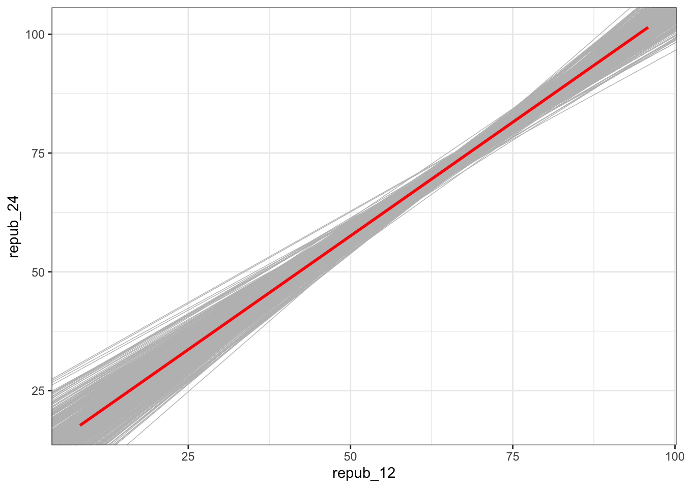
# Approximate sampling distribution of the slope estimate
election_models_50 %>%
ggplot(aes(x = repub_12)) +
geom_density() +
geom_vline(xintercept = 0.957, color = "red")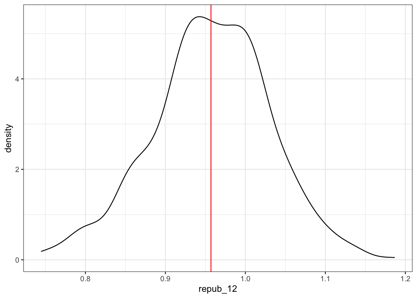
# Approximate standard error of the slope estimate
election_models_50 %>%
summarize(sd(repub_12))
## sd(repub_12)
## 1 0.07349818Reflection: When using a sample of 50 counties, the typical sample estimate of the repub_12 coefficient (slope) is “off” by 0.07 units (2024 vote percentage / 2012 vote percentage), i.e. 0.07 from the actual population slope.
EXAMPLE 4: Approximate the sampling distribution via the CLT
fish <- read_csv("https://Mac-STAT.github.io/data/Mercury.csv")
# Plot the SAMPLE relationship along with the SAMPLE model estimate
fish %>%
ggplot(aes(y = Concen, x = Length)) +
geom_point() +
geom_smooth(method = "lm", se = FALSE)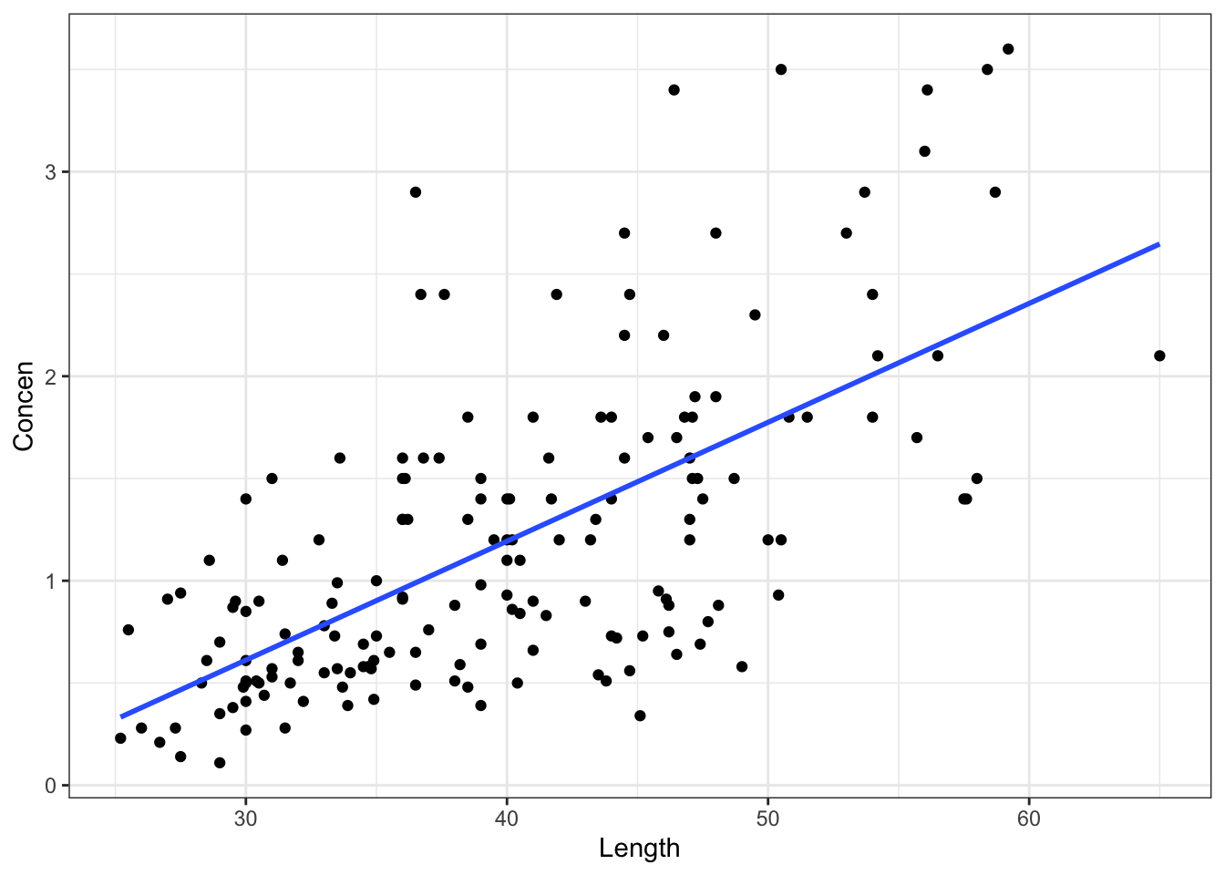
# Obtain the SAMPLE model
fish_model <- lm(Concen ~ Length, data = fish)
coef(summary(fish_model))
## Estimate Std. Error t value Pr(>|t|)
## (Intercept) -1.13164542 0.213614796 -5.297598 3.617750e-07
## Length 0.05812749 0.005227593 11.119359 6.641225e-22We don’t know! We only have a sample of fish.
0.058 (from the model summary table)
0.005
\(\hat{\beta_1} \sim N(\beta_1, 0.005^2)\)
We don’t know!! Since we don’t know what \(\beta_1\) actually is, we don’t know where our estimate falls.
EXAMPLE 5: USE the CLT
0.05
0.010 is 2 standard errors. Since 95% of estimates are within 2 s.e. of \(\beta_1\), 5% are more than 2 s.e. from \(\beta_1\).0.025
0.010 is 2 standard errors. Since 95% of estimates are within 2 s.e. of \(\beta_1\), 5% of more than 2 s.e. away: 2.5% are more than 2 s.e. above \(\beta_1\) and 2.5% are more than 2 s.e. below \(\beta_1\).0.997
0.015 is 3 standard errors and 99.7% of estimates are within 3 s.e. of \(\beta_1\)
Exercise 1: Why “resampling” (replace = TRUE)?
small_sample <- fish %>%
  select(Concen, Length) %>%
  head(4)

small_sample
## # A tibble: 4 × 2
## Concen Length
## <dbl> <dbl>
## 1 1.6 47
## 2 1.5 48.7
## 3 1.7 55.7
## 4 0.73 45.2
lm(Concen ~ Length, data = small_sample)
##
## Call:
## lm(formula = Concen ~ Length, data = small_sample)
##
## Coefficients:
## (Intercept) Length
## -1.82781 0.06532Part a
- These samples always have the same 4 fish, just in different orders.
- Intuition
sample_n(small_sample, size = 4, replace = FALSE)
## # A tibble: 4 × 2
## Concen Length
## <dbl> <dbl>
## 1 0.73 45.2
## 2 1.5 48.7
## 3 1.6 47
## 4 1.7 55.7Part b
- Since the samples are the same, the sample models are always the same
- This doesn’t provide insight into how our results can vary from sample to sample
sample_n(small_sample, size = 4, replace = FALSE) %>%
  with(lm(Concen ~ Length))
##
## Call:
## lm(formula = Concen ~ Length)
##
## Coefficients:
## (Intercept) Length
## -1.82781 0.06532Part c
We sometimes get the same fish more than once!
set.seed(1)sample_n(small_sample, size = 4, replace = TRUE)
## # A tibble: 4 × 2
## Concen Length
## <dbl> <dbl>
## 1 0.73 45.2
## 2 0.73 45.2
## 3 1.5 48.7
## 4 1.6 47The sample models can differ!
sample_n(small_sample, size = 4, replace = TRUE) %>%
  with(lm(Concen ~ Length))
##
## Call:
## lm(formula = Concen ~ Length)
##
## Coefficients:
## (Intercept) Length
## 0.10857 0.02857
Exercise 2: Run a bootstrap simulation
# Set the seed so that we all get the same results
set.seed(155)
# Store the sample models
sample_models_171 <- mosaic::do(500)*(
fish %>%
sample_n(size = 171, replace = TRUE) %>%
with(lm(Concen ~ Length))
)
# Check out the first 6 results
# Make sure that your first Intercept estimate is -1.1802375
head(sample_models_171)
## Intercept Length sigma r.squared F numdf dendf .row .index
## 1 -1.1802375 0.05827521 0.5834448 0.4127396 118.77693 1 169 1 1
## 2 -1.2902917 0.06296431 0.5667005 0.4661328 147.55814 1 169 1 2
## 3 -1.0449945 0.05645232 0.5836492 0.4094752 117.18610 1 169 1 3
## 4 -1.2721884 0.06065800 0.5253640 0.5043690 171.97948 1 169 1 4
## 5 -0.8324804 0.04929179 0.5820092 0.3695009 99.04160 1 169 1 5
## 6 -0.8811652 0.05088282 0.5786866 0.3671583 98.04942 1 169 1 6
Exercise 3: Bootstrap vs CLT sampling distribution
fish %>%
  ggplot(aes(x = Length, y = Concen)) +
  geom_smooth(method = "lm", se = FALSE) +
  geom_abline(data = sample_models_171,
              aes(intercept = Intercept, slope = Length),
              color = "gray", size = 0.25) +
  geom_smooth(method = "lm", color = "red", se = FALSE)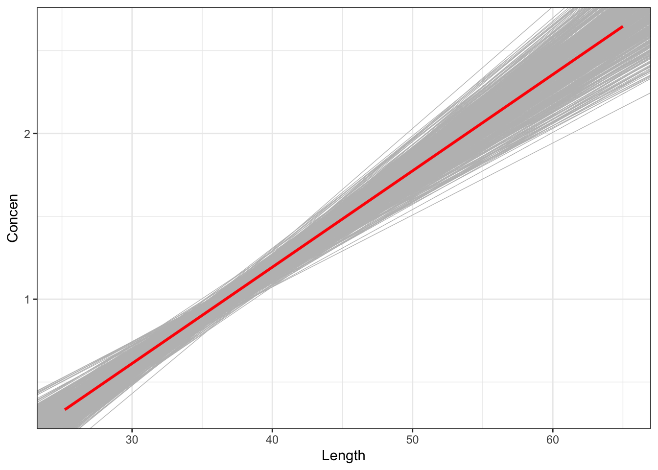
Part a
sample_models_171 %>%
  ggplot(aes(x = Length)) +
  geom_density()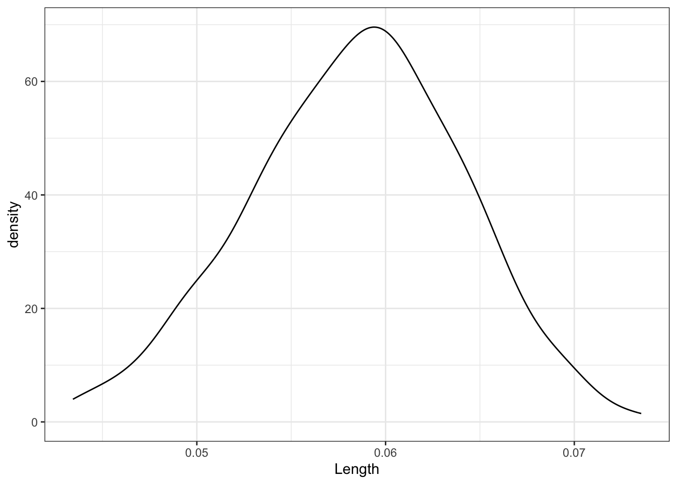
The sampling distribution is symmetric, uni-modal, and shaped like a bell curve!
It is roughly centered at the slope calculated from our entire sample, \(\hat{\beta}_1\)!
Most of the estimates lie within the range 0.04 to 0.075.
Part b
sample_models_171 %>%
summarize(sd(Length))
## sd(Length)
## 1 0.005664586Part c
Yes! The bootstrap distribution is also Normally distributed with an estimated standard error of 0.0057 (close!).
Exercise 4: Increasing sample size – intuition
Intuition
Exercise 5: 500 samples of size n
set.seed(155)
sample_models_50 <- mosaic::do(500)*(
fish %>%
sample_n(size = 50, replace = TRUE) %>%
with(lm(Concen ~ Length))
)
# Check it out
# Make sure that your first Intercept estimate is -1.1602313
head(sample_models_50)
## Intercept Length sigma r.squared F numdf dendf .row .index
## 1 -1.1602313 0.05890697 0.5070761 0.5144595 50.85889 1 48 1 1
## 2 -2.0455811 0.08114633 0.5934863 0.5980898 71.42966 1 48 1 2
## 3 -1.6050619 0.06968133 0.6157918 0.4697283 42.51963 1 48 1 3
## 4 -1.1100806 0.05421924 0.6060071 0.2738796 18.10474 1 48 1 4
## 5 -0.5632098 0.04230700 0.5363858 0.3531607 26.20700 1 48 1 5
## 6 -1.5208830 0.07079659 0.5598511 0.6140689 76.37453 1 48 1 6set.seed(155)
sample_models_20 <- mosaic::do(500)*(
fish %>%
sample_n(size = 20, replace = TRUE) %>%
with(lm(Concen ~ Length))
)
# Check it out
# Make sure that your first Intercept estimate is -2.3961270
head(sample_models_20)
## Intercept Length sigma r.squared F numdf dendf .row .index
## 1 -2.3961270 0.08844853 0.6434716 0.6999700 41.994000 1 18 1 1
## 2 -1.0876343 0.05590552 0.4855417 0.4991518 17.939033 1 18 1 2
## 3 -0.5648239 0.04313415 0.5721530 0.2977556 7.632103 1 18 1 3
## 4 -1.4982809 0.06957034 0.5090352 0.6849533 39.134392 1 18 1 4
## 5 -2.2880439 0.08940596 0.6678969 0.5803712 24.895056 1 18 1 5
## 6 -1.9424474 0.07328658 0.5199477 0.6485854 33.221549 1 18 1 6
Exercise 6: Impact of sample size (part I)
The sample model lines become less and less variable from sample to sample.
# 500 sample models using samples of size 20
fish %>%
  ggplot(aes(x = Length, y = Concen)) +
  geom_smooth(method = "lm", se = FALSE) +
  geom_abline(data = sample_models_20,
              aes(intercept = Intercept, slope = Length),
              color = "gray", size = 0.25) +
  lims(x = c(25, 65), y = c(-1, 5))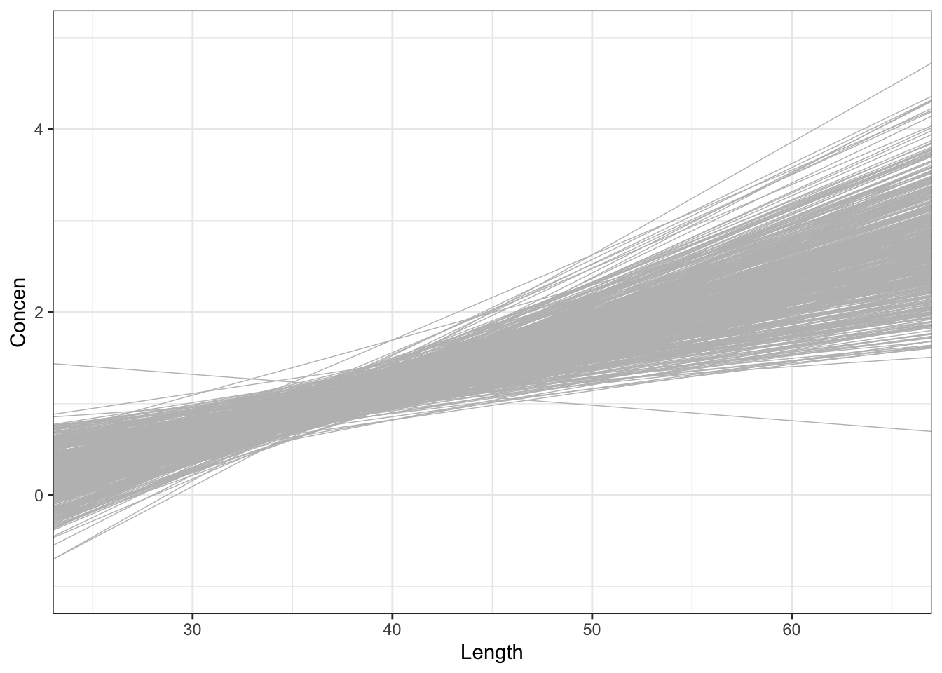
# 500 sample models using samples of size 50
fish %>%
  ggplot(aes(x = Length, y = Concen)) +
  geom_smooth(method = "lm", se = FALSE) +
  geom_abline(data = sample_models_50,
              aes(intercept = Intercept, slope = Length),
              color = "gray", size = 0.25) +
  lims(x = c(25, 65), y = c(-1, 5))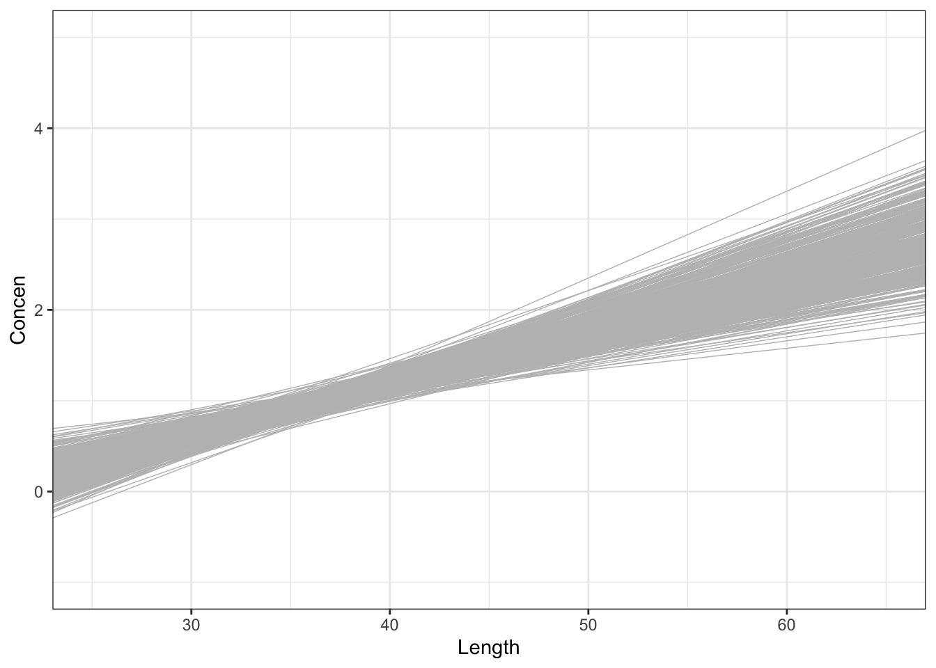
# 500 sample models using samples of size 171
fish %>%
  ggplot(aes(x = Length, y = Concen)) +
  geom_smooth(method = "lm", se = FALSE) +
  geom_abline(data = sample_models_171,
              aes(intercept = Intercept, slope = Length),
              color = "gray", size = 0.25) +
  lims(x = c(25, 65), y = c(-1, 5))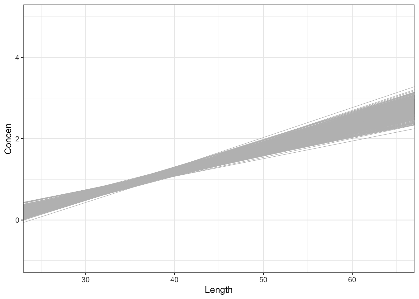
Exercise 7: Impact of sample size (part II)
No matter the sample size, the sample estimates are normally distributed around the same value (here the sample slope since we’re sampling from the sample). But as sample size increases, the variability of the sample estimates decreases.
# 500 sample slopes using samples of size 20
sample_models_20 %>%
  ggplot(aes(x = Length)) +
  geom_density() +
  lims(x = c(-0.01, 0.13), y = c(0, 70))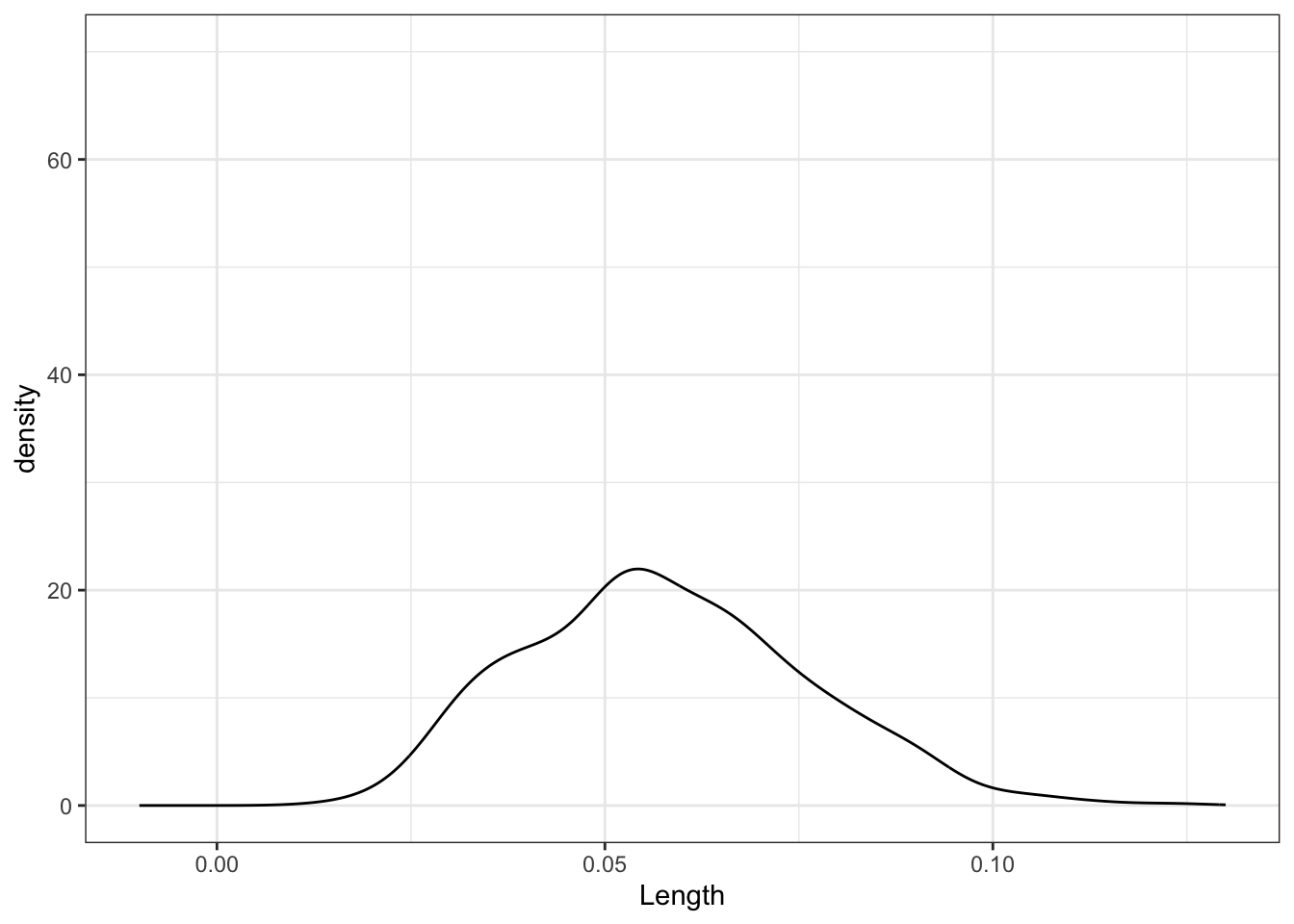
# 500 sample slopes using samples of size 50
sample_models_50 %>%
  ggplot(aes(x = Length)) +
  geom_density() +
  lims(x = c(-0.01, 0.13), y = c(0, 70))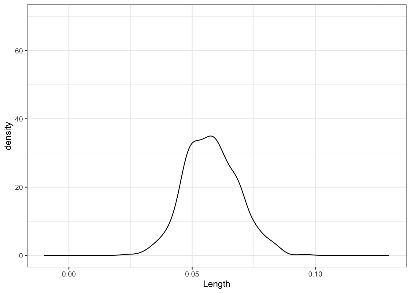
# 500 sample slopes using samples of size 171
sample_models_171 %>%
  ggplot(aes(x = Length)) +
  geom_density() +
  lims(x = c(-0.01, 0.13), y = c(0, 70))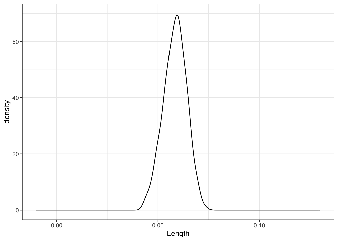
Exercise 8: Properties of sampling distributions
For all sample sizes, the shape of the sampling distribution is roughly normal and is roughly centered around the same location.
As sample size increases:
The average sample slope estimate IS FAIRLY STABLE.
The standard error of the sample slopes DECREASES.Thus, as sample size increases, estimates of the slope become MORE RELIABLE.