10 Interaction
Announcements etc
SETTLING IN
Today is a paper day!
- Put away laptops and phones (in your backpack, not face down on your table).
- You will take notes on paper today. Why?
- To focus on the concepts without getting distracted by R code (which is a necessary tool for, but not the point of, statistical modeling).
- Laptops introduce a lot of distractions to your learning and collaboration.
- After class, you’re encouraged to type up your notes in “10-mlr-interaction-notes.qmd”.
WRAPPING UP
- Type up your activity!
- Upcoming due dates:
- Today = PP 3
- Thursday = CP 9 & Quiz 1 revisions by the start of class.
- Next Tuesday = PP 4 and CP 10
- Continued reminders
- If you don’t finish an activity during class, you should complete it outside of class and check the online solutions.
- Study on an ongoing basis, not just right before quizzes.
Learning goals
- Critically think through whether an interaction term makes sense, or should be included in a multiple linear regression model.
- Write a model formula for a multiple linear regression model with an interaction term.
- Interpret the coefficients in a multiple linear regression model with an interaction term.

Additional resources
References
Let \(Y\) be a response variable and \(X_1\) and \(X_2\) be two predictors. Our previous multiple linear regression models have assumed that the relationship between \(Y\) and \(X_1\) is independent of or unrelated to \(X_2\). In contrast, if the relationship between \(Y\) and \(X_1\) differs depending upon the values / categories of \(X_2\), we say that our 2 predictors \(X_1\) and \(X_2\) interact. In this case we can include an interaction term in our model. Mathematically, this is the product of the 2 predictors:
\[ E[Y | X_1, X_2] = \beta_0 + \beta_1 X_1 + \beta_2 X_2 + \beta_3 X_1*X_2 \]
Warm-up
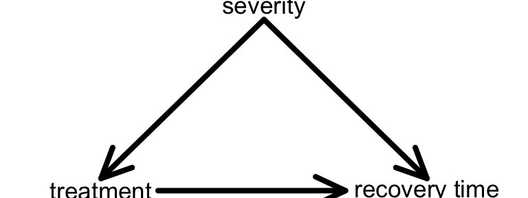
A multiple linear regression model includes more than 1 predictor / explanatory variable X. Different explanatory variables can play different roles. For example, in a model of recovery time (Y) by treatment (predictor of interest \(X_1\)) we should control for symptom severity (confounder \(X_2\)). If we don’t, it might lead to misleading conclusions (eg: that cold treatment A is “better” when really it just looked better because people with less severe symptoms took it).
In a model of wages (Y) by education (predictor of interest \(X_1\)) we should be mindful that this relationship might vary / be impacted by job industry (effect modifier \(X_2\)). Another way to say this is that education and job industry interact. Unless we just want to study one job industry, we need to adjust for this effect modifier by including an interaction term between it and education:

In general
If the relationship between \(Y\) and \(X_1\) differs depending upon the values / categories of \(X_2\), then \(X_1\) and \(X_2\) interact.
EXAMPLE 1: More than 2 predictors
Draw a causal diagram that represents the relationship of wages (Y) with marital status (\(X_1\)) when accounting for age (\(X_2\)), experience (\(X_3\)), and hours worked per week (\(X_4\)). Are any of these confounders or effect modifiers?
EXAMPLE 2: Identify the confounder / effect modifier
It’s our job to identify important confounders and effect modifiers. Context is important!
- Your friend wants to explore the relationship of bikeshare ridership among casual riders with temperature.
- Is weekend status a potential confounder or effect modifier in this relationship?
- Represent your ideas using a causal diagram.

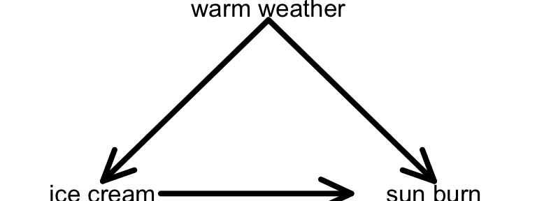
- Another friend claims that ice cream causes sun burns, noting that sun burn rates increase as ice cream sales increase. They are mistaken!
- What important variable did they not consider in their analysis?
- Is this a potential confounder or effect modifier?
- Represent your ideas using a causal diagram.
EXAMPLE 3: Interaction or no interaction?
In addition to context, we can use plots to help identify potential interactions among our predictors, i.e. potential effect modifiers.
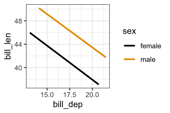
- In a model of penguin bill length, is there a “notable” interaction between bill depth and sex? Provide evidence and explain your answer in context.
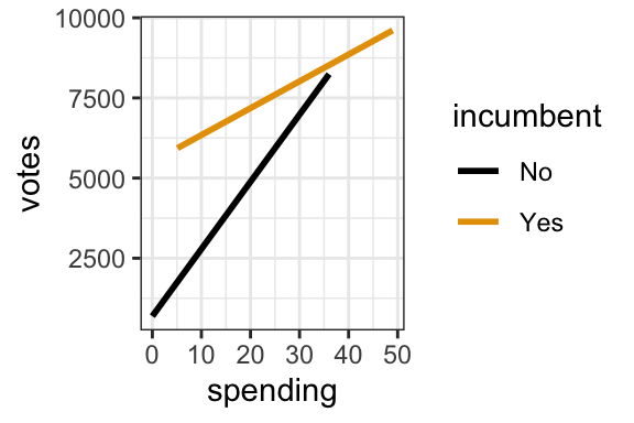
- Benoit and Marsh (2008) explore the 2002 Irish Dail elections, Ireland’s version of the U.S. House of Representatives. Specifically, they explore how the number of
votesa candidate received is associated with their campaignspending(in 1,000s of Euros) and theirincumbentstatus:Yes= candidate is an incumbent (they are running for RE-election), orNo. Is there a “notable” interaction between campaign spending and incumbent status? Provide evidence and explain your answer in context.
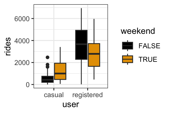
- In a model of bikeshare ridership, is there a “notable” interaction between weekend and user status (whether a user is a casual or registered rider)? Provide evidence and explain what your answer means in context.
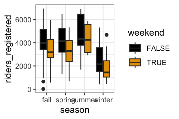
- In a model of bikeshare ridership among registered riders, is there a “notable” interaction between weekend status and season? Provide evidence and explain your answer in context.
EXAMPLE 4: Implementing interaction terms
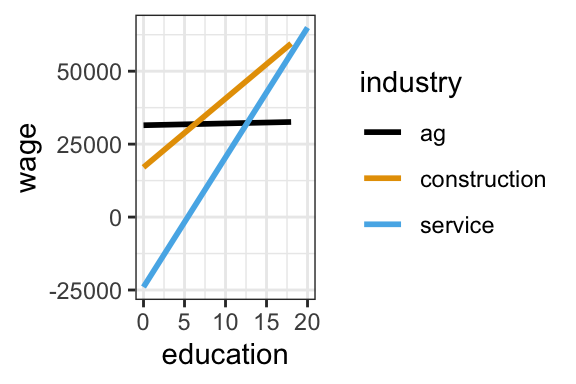
Let’s get into the technical details of effect modifiers / including interaction terms in our models. Below is a model of wage by education, industry, and an interaction between education and industry. The industries in our analysis are: ag, construction, service. Identify what part of our lm() code is new:
cps <- read_csv("https://mac-stat.github.io/data/cps_2018.csv") %>%
  filter(industry %in% c("ag", "construction", "service"))
wage_model <- lm(wage ~ industry * education, cps)
coef(summary(wage_model))
## Estimate Std. Error t value Pr(>|t|)
## (Intercept) 31475.87521 17897.892 1.75863593 0.078709335
## industryconstruction -14427.01189 20594.475 -0.70052828 0.483634737
## industryservice -55462.76415 18584.852 -2.98429945 0.002858015
## education 61.95396 1631.542 0.03797265 0.969711223
## industryconstruction:education 2295.51232 1838.280 1.24872836 0.211831318
## industryservice:education 4384.72036 1674.157 2.61906115 0.008847667
EXAMPLE 5: Differences by industry
The estimated model formula, rounded, is written out and visualized below:
E[wage | ed, industry] = 31476 - 14427 construction - 55463 service + 62 ed + 2296 ed*construction + 4385 ed*service
Prove the related sub-model formulas for 2 of the 3 industries:
ag: \(\text{E[wage | education]} = 31476 + 62 \text{ education}\)service: \(\text{E[wage | education]}= -23987 + 4447 \text{ education}\)
Try to answer the following using only the model formula:
In what industry do average wages increase the most per additional year of education? What is that rate of increase?
In what industry do average wages increase the least per additional year of education? What is that rate of increase?
EXAMPLE 6: Interpretation
Interpret the following model coefficients and represent them on the plot above. Remember: Use non-causal language, include units, and talk about averages rather than individual cases.
Intercept coefficient = 31476
This is the expected wage for someone with 0 years of education in…industryservicecoefficient = -55463
The expected wage for someone with 0 years of education is -55462.76 lower in…educationcoefficient = 62
For every extra year of education, the average wage increases by $61.95 in…education:industryservice= 4385
The increase in average wage with every extra year of education is…Note that we didn’t and can’t “hold constant” education when interpreting the industry coefficient, or vice versa. Why?
Exercises
GOAL: Explore interaction terms among various types of variables, categorical and/or quantitative!
Exercise 1: Interaction between 1 Q & 1 C
In exploring the relationship of a candidate’s votes with their campaign spending (in 1,000s of Euros), we must consider their incumbent status (an effect modifier):

The corresponding estimated model formula is
E[votes | spending, incumbent] = 691 + 209.7 spending + 4814 incumbentYes - 125.9 spending*incumbentYes
vote_model <- lm(votes ~ spending * incumbent, campaigns)
coef(summary(vote_model))
##                        Estimate Std. Error   t value     Pr(>|t|)
## (Intercept)            690.5169  168.60193  4.095546 4.978190e-05
## spending               209.6578   13.54984 15.473080 9.189028e-44
## incumbentYes          4813.8932  472.40711 10.190137 4.042033e-22
## spending:incumbentYes -125.8706   25.63343 -4.910409 1.265704e-06
Part a
Write out the sub-model formulas for incumbents and non-incumbents. Simplify / combine like terms.
For non-incumbents: E[votes | spending] =
For incumbents: E[votes | spending] =
Part b
Interpret the (Intercept) and incumbentYes coefficients, 691 and 4814, in context.
Part c
Interpret the spending and interaction (spending:incumbentYes) coefficients, 209.7 and -125.9, in context. Pro tip: First focus on the signs of these coefficients, then interpret the details.
Exercise 2: But is it meaningful?
When interpreting coefficients, we should reflect on whether they are scientifically meaningful. That is, is the magnitude of the coefficient meaningful or notable in the context of the analysis?
Part a
Is the spending coefficient of 209.66 scientifically meaningful? That is, is the scale of the increase in expected votes with spending among non-incumbents “notable”?
Part b
Is the interaction term between incumbent status and spending scientifically meaningful? That is, is the difference in the rate of increase in votes with spending for incumbents vs non-incumbents notable?
Exercise 3: Interaction between 2 C
Next, let’s explore the relationship of daily bike ridership (Y) and whether a user is a casual or registered rider and whether the day falls on a weekend. We’ll use the same bike data as before, but wrangled into a format that allows us to answer this question:
head(new_bikes, 3)
## # A tibble: 3 × 4
##   weekend temp_actual user       rides
##   <fct>         <dbl> <chr>      <dbl>
## 1 TRUE           57.4 casual       331
## 2 TRUE           57.4 registered   654
## 3 TRUE           58.8 casual       131
In the warm-up, we noted that user and weekend status predictors interact, i.e. the relationship of ridership with weekend status varies by user group:
new_bikes %>%
  ggplot(aes(y = rides, x = user, fill = weekend)) +
  geom_boxplot()
Part a
The estimated model of this relationship is
E[rides | weekend, user] = 625 + 777 weekendTRUE + 3300 userregistered - 1714 weekendTRUE*userregistered
bike_model <- lm(rides ~ weekend * user, new_bikes)
coef(summary(bike_model))
##                              Estimate Std. Error   t value      Pr(>|t|)
## (Intercept)                  503.4352   59.39416  8.476173  7.561991e-17
## weekendTRUE                  718.8551  110.96258  6.478356  1.407175e-10
## userregistered              3136.1891   83.99603 37.337348 1.700783e-196
## weekendTRUE:userregistered -1535.5246  156.92479 -9.785099  1.013828e-21
Use this model to make 2 predictions:
Predict casual ridership on a weekday =
Predict registered ridership on a weekend =
Part b
Use the appropriate coefficient estimate(s) to answer the following. (This is not easy! The boxplots can help you assess whether your answers make sense!)
On weekdays, how many more registered vs casual riders would we expect?
Among casual riders, how many more riders would we expect on a weekend vs weekday?
Among registered riders, how many fewer riders would we expect on a weekend vs weekday? NOTE: The answer is NOT 1714.
Among casual riders, what’s the expected ridership on a weekday?
Exercise 4: Interactions between 2 Q
Finally, let’s explore the relationship of price (Y) with 2 quantitative predictors: the mileage and age of a used car. In doing so, it’s important to keep in mind that mileage and age interact: the relationship of price with mileage differs depending upon the age of the car.
Part a
The lines below represent the relationship of price with mileage for different aged cars: 0 years old (solid), 10 years old (dashed), and 20 years old (dotted).
# Don't worry about this code
cars <- read_csv("https://mac-stat.github.io/data/used_cars.csv") %>%
  mutate(mileage = milage %>% str_replace(",","") %>% str_replace(" mi.","") %>% as.numeric(),
         price = price %>% str_replace(",","") %>% str_replace("\\$","") %>% as.numeric(),
         age = 2025 - model_year) %>% # 2025 so that yr. 2024 cars are one year old
  select(-milage)

cars %>%
  ggplot(aes(y = price, x = mileage)) +
  geom_abline(aes(intercept = 90965, slope = -0.66)) +
  geom_abline(aes(intercept = 64314, slope = -0.46), linetype = 2) +
  geom_abline(aes(intercept = 37664, slope = -0.26), linetype = 3) +
  lims(x = c(0, 100000), y = c(0, 100000))
Discuss in words how the relationship between price and mileage varies by the aged of a used car.
Part b
The model of price by mileage and age, with an interaction term, is represented by:
E[price | mileage, age] = \(\beta_0\) + \(\beta_1\) mileage + \(\beta_2\) age + \(\beta_3\) mileage*age
Using the above plot as a guide, what are the signs of the 4 \(\beta\) coefficients (+/-)?
Part c
Below is the actual model summary table:
car_model <- lm(price ~ mileage * age, cars)
coef(summary(car_model))
##                  Estimate   Std. Error   t value     Pr(>|t|)
## (Intercept) 90964.8342889 1.838484e+03  49.47817 0.000000e+00
## mileage        -0.6557997 3.089039e-02 -21.22989 7.186318e-95
## age         -2665.4395549 2.013130e+02 -13.24028 3.389030e-39
## mileage:age     0.0243140 2.089504e-03  11.63625 8.401747e-31
Use this to:
Check your answer to Part b.
Specify the sub-model formula of E[price | mileage] for 0 year old (new) cars.
Specify the sub-model formula of E[price | mileage] for 10 year old (used) cars.
Exercise 5: Cars continued
Part a
Interpret the mileage coefficient, -0.66, in context. Think: This tells us about the rate of decrease of price with mileage for cars of what age?!
Part b
Interpret the interaction coefficient, 0.02, in context. Think: What does it tell us about the rate of decrease of price with mileage as cars age?!
Part c
To check out plots of the raw data behind this model, visit the qmd or online manual. Neither of the options are very helpful (it’s tough to visualize 3D relationships, especially in the presence of interaction)!
cars %>%
  ggplot(aes(x = mileage, y = price, col = age)) +
  geom_point(alpha = 0.5) +
  scale_color_viridis_c(option = "H") # a fun, colorblind-friendly palette!
# BONUS: visualize this in "3D"
library(plotly)
cars %>%
plot_ly(x = ~mileage, y = ~age, z = ~price, color = ~price,
type = "scatter3d",
mode = "markers",
marker = list(size = 5, colorscale = "Viridis"))
Next steps
You’re encouraged to type up your written notes in the provided qmd! This is a good way to study.
Solutions
EXAMPLE 2: Identify the confounder / effect modifier
- Weekend status is an effect modifier: the relationship of ridership with temperature varies by weekend / weekday:

- Warm weather is a potential confounder. The warmer the weather, the more the ice cream sales and the more incidences of sun burn.
EXAMPLE 3: Interaction or no interaction?
No. The lines are parallel – the decrease of bill length with bill depth is similar for the different species.
Yes. The lines are not parallel – the increase of votes with spending is quicker for non-incumbents.
Yes. The relationship between rides and weekend status varies by user status – ridership tends to be higher on weekends for casual riders, but lower on weekends for registered riders.
No. The relationship between rides and weekend status is similar in each season – ridership tends to be lower on weekends (and the diff in ridership on weekends vs weekdays is similar in each season).
EXAMPLE 4: Implementing interaction terms
We use * instead of + between our predictors.
##                                    Estimate Std. Error     t value    Pr(>|t|)
## (Intercept)                     31475.87521  17897.892  1.75863593 0.078709335
## industryconstruction           -14427.01189  20594.475 -0.70052828 0.483634737
## industryservice                -55462.76415  18584.852 -2.98429945 0.002858015
## education                          61.95396   1631.542  0.03797265 0.969711223
## industryconstruction:education   2295.51232   1838.280  1.24872836 0.211831318
## industryservice:education        4384.72036   1674.157  2.61906115 0.008847667
EXAMPLE 5: Differences by industry

- .
ag: E[wage | education] = 31476 + 62 education
E[wage | education, industry]
= 31476 + 62 education - 14427*0 - 55463*0 + 2296 education*0 + 4385 education*0
= 31476 + 62 education - 0 - 0 + 0 + 0service: E[wage | education] = -23987 + 4447 educationE[wage | education, industry]
= 31476 + 62 education - 14427*0 - 55463*1 + 2296 education*0 + 4385 education*1
= 31476 + 62 education - 0 - 55463 + 0 + 4385 education
= (31476 - 55463) + (62 + 4385) education
- service: 4447 (62 + 4385)
ag: 62
EXAMPLE 7: Interpretation
Intercept coefficient = 31476
This is the expected wage for someone with 0 years of education in the ag industry.industryservicecoefficient = -55463
The expected wage for someone with 0 years of education is -55462.76 lower in the service industry than in the ag industry.educationcoefficient = 62
For every extra year of education, the average wage increases by $61.95 in the ag industry.education:industryservice= 4385
The increase in average wage with every extra year of education is $4385/year higher in the service industry than in the ag industry.The difference in wages by industry differs (is not constant) depending upon the years of education.
Exercise 1: Interaction between 1 Q & 1 C
Part a
For non-incumbents: E[votes | spending] = 690.5 + 209.7 spending
For incumbents: E[votes | spending] = 690 + 4813.9 + 209.7 spending - 125.9 spending = 5503.9 + 83.8 * spending
Part b
If 0 Euros are spent, we’d expect a non-incumbent to get 691 votes and an incumbent to get 4814 votes more than that (hence 691 + 4814 = 5505 votes).
Part c
For every extra 1,000 Euros spent, the expected number of votes for a non-incumbent increases by 210. The increase in expected votes per 1,000 Euros spent for an incumbent is 84, 126 less than for a non-incumbent.
Exercise 2: But is it meaningful?
Part a
It seems so! 210 votes seems like quite a bit on the scale of the data shown here.
Part b
It seems so! The difference in 84 and 210 votes per 1000 Euros is pretty big. The interaction term gives us the additional information that spending has less of an effect on number of votes for incumbents than it does for challengers, which is particularly meaningful if you are a campaign manager!
Exercise 3: Interaction between 2 C
Part a
# Predict casual ridership on a weekday
625 + 777*0 + 3300*0 - 1714*0*0

# Predict registered ridership on a weekend
625 + 777*1 + 3300*1 - 1714*1*1
Part b
- 3300
- 777
- 937 (777-1714)Among registered riders, how many fewer riders would we expect on a weekend vs weekday? NOTE: The answer is NOT 1714.
- 625
Exercise 4: Interactions between 2 Q
Part a
Prices tend to be decrease with both mileage and age. The decrease of expected price with mileage is less steep the older the cars.
Part b
\(\beta_0\): positive, since the intercept is the average price for a car with zero miles that is brand new.
\(\beta_1\): negative, since the more miles a new car has, the cheaper it should be
\(\beta_2\): negative, since the intercept of the lines seems to decrease with age (black -> blue -> green)
\(\beta_3\): positive, since the slope of the lines seems to increase with age (black -> blue -> green)
Part c
- 0 year old used cars: E[price | mileage] = 90965 - 0.66 mileage
- 10 year old used cars:
E[price | mileage]
= 90965 - 0.66 mileage - 2665(10) + 0.02(10) mileage
= 90965 - 0.66 mileage - 26650 + 0.2 mileage = 64315 - 0.46 mileage
Exercise 5: Cars continued
Part a
For 0 year old cars, the expected price decreases by $0.66 for every additional mile.
Part b
The overall decrease in the expected price per mile is $0.02 less for each additional year old the car is. (That is, the slope of price vs mileage is still negative, but less negative as age increases.)