18 Confidence intervals

Announcements etc

SETTLING IN

Sit with people that are NOT in your project group. If there’s extra time after the activity, you will work on PP 6 not the project.
Today is a paper day. For future reference you can access the qmd here: “18-confidence-intervals-notes.qmd”.
Hand in Quiz 2 revisions if you have them. (The latest these will be accepted for credit is Tuesday 11/18, 1 week after the deadline.)

WRAPPING UP

Upcoming due dates:

Thursday
- PP 6
Next week
- Tuesday
  - Last chance to hand in Quiz 2 revisions (due at the beginning of class)
  - CP 15
- Thursday
  - PP 7
The week after that!
- Tuesday
  - Project Milestone 2
  - Project work day. Can’t be here? Consider Zooming in with your group. At minimum, coordinate a plan with them.
Related but unrelated: MSCS events calendar

Learning goals

Construct (approximate) confidence intervals by hand using the 68-95-99.7 rule
Construct exact confidence intervals in R
Interpret confidence intervals in context by referring to the coefficient of interest
Use confidence intervals to make statements about whether there appear to be true population relationships, changes, and differences

Additional resources

Required video

Introduction to Confidence Intervals

Optional

Read: Section 7 Introduction, 7.1, 7.2 (stop when you get to 7.2.4.3 Confidence Intervals for Prediction) in the STAT 155 Notes
Watch (after class): Confidence Intervals: Construction and Interpretation

References

Set-up

\(\beta\) = some population parameter (e.g. a model coefficient)
\(\hat{\beta}\) = a sample estimate of \(\beta\)
\(\text{s.e.}(\hat{\beta})\) = the standard error of \(\hat{\beta}\) (essentially the typical error for an estimate calculated from a sample of our size n)

Central Limit Theorem (CLT): Approximating the sampling distribution

The collection of possible \(\hat{\beta}\) calculated from different samples of size n (i.e. the sampling distribution of \(\hat{\beta}\)) is Normally distributed around \(\beta\):

\[ \hat{\beta} \sim N(\beta, \; \text{s.e.}(\hat{\beta})^2) \]

Confidence interval for \(\beta\)

To communicate and contextualize the potential error in \(\hat{\beta}\), we can calculate a confidence interval (CI) for \(\beta\). This CI:

reflects the potential error in \(\hat{\beta}\); while
providing a range of plausible values for \(\beta\), i.e. an interval estimate; thus
allows us to draw fair conclusions about the population using data from our sample!

Using the CLT, an approximate 95% confidence interval for \(\beta\) can be calculated by the formula below. (More precise calculations are provided in RStudio.)

\[ \hat{\beta} \pm 2 \text{s.e.}(\hat{\beta}) \]

What does “95% confidence” mean?!

Important nuances:
- \(\beta\) is “fixed”, i.e. not random. There’s a fixed, “true” value of \(\beta\), we just don’t know what it is. Thus we can’t make probability statements about \(\beta\).
- \(\hat{\beta}\) is random (it varies from sample to sample, depending upon what sample we happen to get). Thus we can make probability statements about \(\hat{\beta}\).
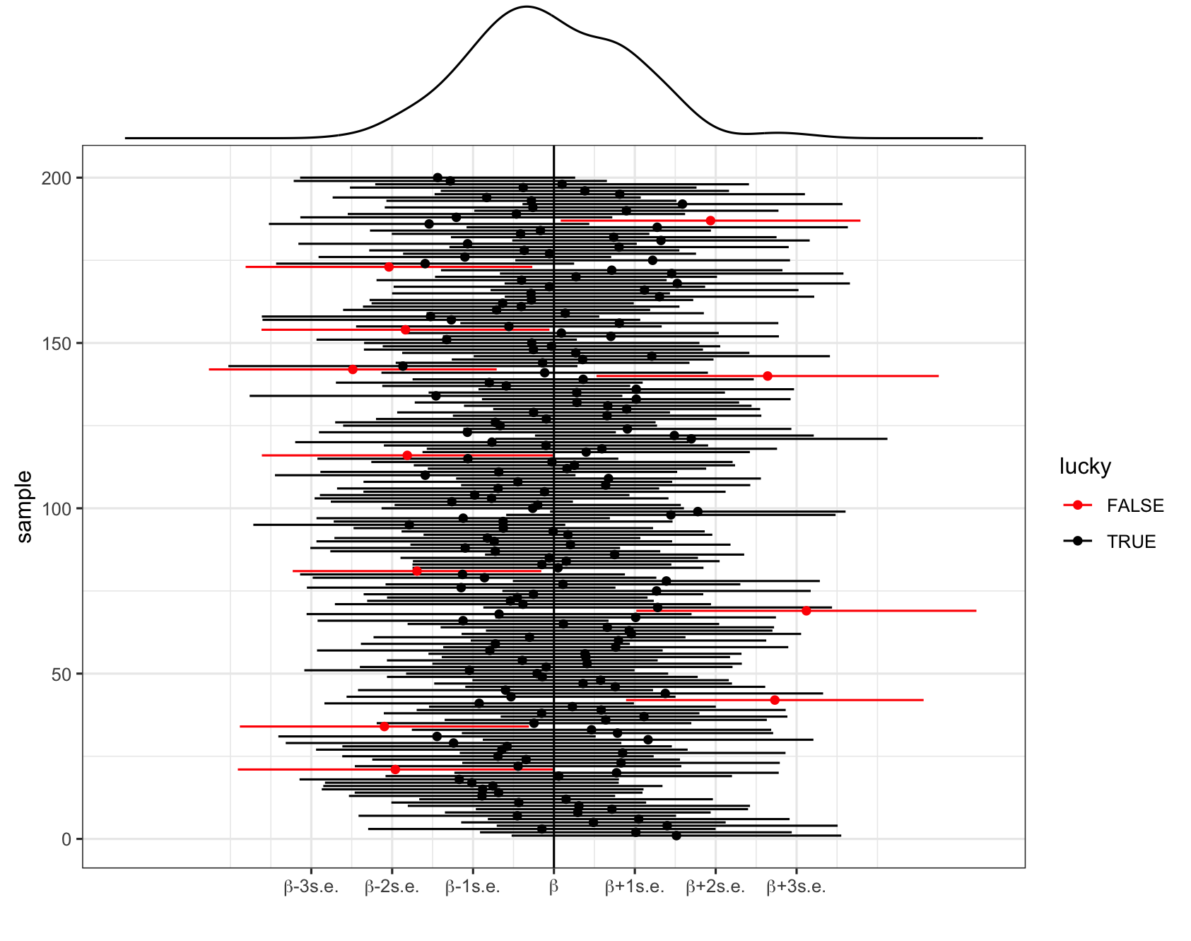
Thus “95% confidence” references the randomness and variability in \(\hat{\beta}\) and the interval construction process, not \(\beta\): 95% of all possible samples will produce 95% CIs that contain the true \(\beta\) value.
In pictures: 200 different 95% CIs for \(\beta\) calculated from 200 different samples. Each sample produces a different estimate \(\hat{\beta}\) (dot) hence a different 95% CI for \(\beta\) (horizontal line). Roughly 95% of these contain \(\beta\) (the black intervals) and roughly 5% do not (the red intervals).

Interpreting a CI

Let (a, b) represent the 95% CI for \(\beta\).

Correct: We are 95% confident that \(\beta\) is between a and b.
Incorrect: There’s a 95% chance that \(\beta\) falls between a and b.
- Nope! \(\beta\) is either in there, or it isn’t. No probability involved.
- It is either in the interval or not, so the probability is 1 or 0.
Incorrect: There’s a 95% chance that sample estimate \(\hat{\beta}\) is between a and b.
- Nope! We have no uncertainty about \(\hat{\beta}\) – we know exactly what it is and it’s always in the interval by construction.

Exercises

Goals

Build up our confidence with confidence intervals (!) by starting with some familiar data and the simple linear regression setting.
Explore how to use CIs to assess the “significance” of our sample results.

Exercise 1: Standard errors

In the first set of exercises, we’ll model the time it takes to complete a mountain hike. To begin, let’s explore the relationship of completion time (in hours) by hike length (in miles):

E[time | length] = \(\beta_0\) + \(\beta_1\) length

A sample estimate of this population model, obtained using our data on hiking trails in the Adirondack mountains, is below:

E[time | length] = \(\hat{\beta}_0\) + \(\hat{\beta}_1\) length = 2.048 + 0.684 length

# Import the data & load important packages
library(tidyverse)
peaks <- read.csv("https://mac-stat.github.io/data/high_peaks.csv")

# Model the relationship
peaks_model_1 <- lm(time ~ length, data = peaks)
coef(summary(peaks_model_1))

# Visualize the relationship
peaks %>% 
  ggplot(aes(y = time, x = length)) + 
  geom_point() + 
  geom_smooth(method = "lm")

Part a

Since \(\hat{\beta}_1 = 0.684\), we estimate that the expected hiking time increases by 0.684 for every additional mile in hiking length. Report and interpret \(s.e.(\hat{\beta}_1)\), the standard error of this estimate.

Part b

Considering context, units, and scale of our data (as illustrated in the plot), do you think this is a small, moderate, or large amount of error? (Mainly, do you think our slope estimate is pretty accurate or does the standard error make you skeptical?)

Exercise 2: Constructing a CI

Continue to let \(\beta_1\) be the “true” population length coefficient, and \(\hat{\beta}_1 = 0.684\) be our sample estimate of \(\beta_1\).

Part a

\(\hat{\beta}_1\) simply provides a point estimate, or our single best guess, of \(\beta_1\). To also produce an interval estimate, use the 68-95-99.7 Rule to approximate a 95% CI for \(\beta_1\).

Part b

We can calculate a more accurate CI by applying the confint() function to our model. Your approximation from Part a should be close!

confint(peaks_model_1, level = 0.95)

Exercise 3: Interpreting the CI

Part a

Interpreting the CI for \(\beta_1\) in context requires that we can interpret \(\beta_1\) itself! So how can we interpret \(\beta_1\) (in general, without assuming a specific value for the unknown \(\beta_1\))?

\(\beta_1\) measures the expected completion time for hikes that are 0 miles long
\(\beta_1\) measures the difference in the expected completion time for hikes that long vs hikes that aren’t long
\(\beta_1\) measures the change in the expected completion time for each additional 1 mile in length

Part b

Per the previous exercise: “We are 95% confident that \(\beta_1\) is between 0.56 and 0.81”. Interpret this CI in context, drawing on your answer to Part a.

Exercise 4: Changing the confidence level

Our 95% CI for \(\beta_1\) is (0.560, 0.808). What would happen if we changed the confidence level?!

Part a

If we lower our confidence level from 95% to 68%, only 68% of samples would produce 68% CIs that cover \(\beta_1\). Intuitively, would the 68% CI be narrower or wider than a 95% CI?

Part b

Use the 68-95-99.7 Rule to approximate the 68% CI for \(\beta_1\).

Part c

What if we wanted to be VERY VERY confident that our CI covered \(\beta_1\)? Use the 68-95-99.7 Rule to approximate the 99.7% CI for \(\beta_1\).

Part d

What if we wanted to be 100% confident that our CI covered \(\beta_1\)?! What do you think the CI would have to be?! (Use logic – the 69-95-99.7 Rule doesn’t help in this scenario.)

Part e

Check your answers to Parts b-d using confint(). (Your answers should be close but not exact.)

confint(peaks_model_1, level = 0.68)
confint(peaks_model_1, level = 0.997)
confint(peaks_model_1, level = 1)

Exercise 5: Trade-offs

Summarize the trade-offs in increasing confidence levels, say from 95% to 99.7%, for a CI of some population parameter \(\beta\).

Part a

Choose the correct words for both statements. As confidence level increases…

the percent of CIs that cover \(\beta\)…increases / decreases / stays the same; and
the width of the CI…increases / decreases / stays the same.

Part b

Why is a very wide CI less useful than a narrower CI? For example, what if a pollster reported with 99.7% confidence that the support for “Candidate A” in an upcoming election is between 5% and 85%?

Part c

Practitioners typically use a 95% confidence level. Comment on why you think this is.

Exercise 6: Using CIs to test hypotheses

Recall our population model of interest:

E[time | length] = \(\beta_0\) + \(\beta_1\) length

A typical research question here might be whether, in the population of hikes, there’s a “significant” relationship between hiking time and length (i.e. \(\beta_1 \ne 0\)). Though our sample estimate suggested there’s a positive relationship (\(\hat{\beta}_1 = 0.684\)), there’s error in this estimate. So…does our sample still suggest a relationship after accounting for this potential error?!

Part a

The sample model is plotted below along with confidence bands that reflect its potential error. Based on this plot alone, what do you think? When accounting for the potential error in our sample model, do we have evidence of a “significant” relationship between hiking time and length?

peaks %>% 
  ggplot(aes(y = time, x = length)) + 
  geom_point() + 
  geom_smooth(method = "lm")

Part b

Recall that our 95% CI for \(\beta_1\) was roughly \((0.560, 0.808)\). Using this CI alone, do we have evidence of a “significant” relationship between hiking time and length?

Part c

To answer Parts a and b, you had to make up some “rules” for using plots and CIs to evaluate the significance of \(\beta_1\). In general, what were these rules?!

If (something about the plot), then our sample data provides evidence of a “significant” relationship between Y and X.
If (something about the CI), then our sample data provides evidence of a “significant” relationship between Y and X.

Part d

Your work above suggests that there’s a statistically significant association between hiking time and length. This merely suggests that an association exists (\(\beta_1 \ne 0\)). It does not necessarily mean that the magnitude of the association is meaningful, or practically significant, in context.

Do you think that the association between hiking time and length is also practically significant? Mainly, in the context of hiking, is the magnitude of the association (an increase between 0.560 and 0.808 hours in expected hiking time for every 1-mile increase in length) actually meaningful?

Exercise 7: time versus elevation

Next, let’s explore the relationship between the completion time and maximum elevation of a hike (in feet):

E[time | elevation] = \(\beta_0\) + \(\beta_1\) elevation

We can gain insight into this relationship using our sample data:

# Model the relationship
peaks_model_2 <- lm(time ~ elevation, data = peaks)

# Get confidence intervals
confint(peaks_model_2, level = 0.95)

# Plot the sample model
ggplot(peaks, aes(y = time, x = elevation)) + 
  geom_point() + 
  geom_smooth(method = "lm")

What can we conclude from both the CI for \(\beta_1\) and the confidence bands in the plot above?

Exercise 8: time versus rating

Next, let’s explore the relationship between the completion time and hike rating (difficult, easy, or moderate):

E[time | rating] = \(\beta_0\) + \(\beta_1\) ratingeasy + \(\beta_2\) ratingmoderate

PAUSE: Before analyzing this model, pause to reflect on what \(\beta_0\), \(\beta_1\), and \(\beta_2\) mean in this context. We can gain insight into these coefficients using our sample data:

# Visualize the relationship
ggplot(peaks, aes(y = time, x = rating)) + 
  geom_boxplot()

# Model the relationship
peaks_model_3 <- lm(time ~ rating, data = peaks)

# Obtain CIs for the model coefficients
confint(peaks_model_3)

Part a

How can we interpret the confidence interval for \(\beta_2\), the ratingmoderate coefficient: (-5.92, -3.19)? We’re 95% confident that…

the average completion time of a moderate hike is between 3.19 and 5.92 hours
the average completion time of a moderate hike is between 3.19 and 5.92 hours less than that of a difficult hike
the average completion time of moderate hikes in our sample was between 3.19 and 5.92 hours less than that of difficult hikes in our sample

Part b

How can we interpret the confidence interval for the intercept \(\beta_0\): (13.8, 16.2)? We’re 95% confident that…

the average completion time of a hike with a 0 rating is between 13.8 and 16.2 hours.
the average completion time of a difficult hike is between 13.8 and 16.2 hours.
the average completion time of a hike is between 13.8 and 16.2 hours.
the average completion time of a difficult hike is between 13.8 and 16.2 hours more than that of an easy hike.

Part c

Based on the CIs, does our sample data provide evidence of a “significant” relationship between hiking time and rating?

Exercise 9: Multiple logistic regression REVIEW

Let’s turn our attention to weather in 3 Australia locations, Hobart, Uluru, and Wollongong: When controlling for location, is today’s 9am humidity level (0-100%) a “significant” predictor of whether or not it will rain tomorrow? The following population model represents this relationship:

log(odds of rain_tmrw) = \(\beta_0\) + \(\beta_1\) locationUluru + \(\beta_2\) locationWollongong + \(\beta_3\) humidity9am

Below we build a sample model using a sample of 500 data points:

# NOTE: We'll take a sub-sample of 500 days for TEACHING PURPOSES ONLY
# In practice, we'd use all data in our sample :)
set.seed(155)
weather <- read_csv("https://mac-stat.github.io/data/weather_3_locations.csv") %>% 
  mutate(rain_tmrw = (raintomorrow == "Yes")) %>% 
  sample_n(size = 500, replace = FALSE)

# Build the sample model
weather_model_1 <- glm(rain_tmrw ~ location + humidity9am, data = weather, family = "binomial")
coef(summary(weather_model_1))

# Exponentiate the coefficients
exp(-4.231)
exp(-0.504)
exp(0.040)

Part a

Why are we using logistic regression?

Part b

Interpret \(\hat{\beta}_0\), the estimated intercept, on the odds scale. Circle any option that’s correct! On a day with 0 humidity at 9am in Hobart…

The odds of rain are 0.015.
The chance of rain is 0.015.
The chance of rain is 1.5% as high as the chance of no rain.
The odds of rain increase by 0.15%.

Part c

Interpret \(\hat{\beta}_1\), the estimated locationUluru coefficient, on the odds scale. When controlling for 9am humidity levels…

the odds of rain are 0.60 in Uluru.
the odds of rain are 60% higher in Uluru than in Hobart.
the odds of rain in Uluru are 60% as high as (hence 40% lower than) the odds in Hobart.
the chance of rain in Uluru is 60% as high as (hence 40% lower than) the chance that it doesn’t rain.

Part d

Interpret \(\hat{\beta}_3\), the estimated humidity9am coefficient, on the odds scale. When controlling for location…

the odds of rain increase by 4% for every additional 1-percentage point increase in 9am humidity.
the odds of rain increase by 1.04 for every additional 1-percentage point increase in 9am humidity.
the odds of rain are 1.04.

Exercise 10: Inference for logistic regression

Let’s focus on \(\beta_1\), the “true” locationUluru coefficient. In the previous exercise, we estimated \(\beta_1\) to be -0.504 (or 0.604 on the odds scale).

Part a

On the log(odds) scale, the 95% CI for \(\beta_1\) is roughly

\[ -0.504 \pm 2*0.414 = (-1.332, 0.324) \]

More accurately:

confint(weather_model_1)

What can we conclude?

We do not have evidence that the chance of rain significantly differs in Uluru and Hobart.
We do not have evidence that the chance of rain significantly differs in Uluru and Hobart when controlling for 9am humidity (i.e. when the 9am humidity is the same in both locations).
We do have evidence that the chance of rain significantly differs in Uluru and Hobart.
We do have evidence that the chance of rain significantly differs in Uluru and Hobart when controlling for 9am humidity.

Part b

We can also convert the 95% CI to the odds scale by exponentiating the limits:

\[ (e^{-1.332}, e^{0.324}) = (0.264, 1.38) \]

More accurately:

exp(confint(weather_model_1))

What can we conclude?

We do not have evidence that the chance of rain significantly differs in Uluru and Hobart when controlling for 9am humidity.
We do have evidence that the chance of rain significantly differs in Uluru and Hobart.

Part c

Your answers to Parts a and b should agree! Changing between the log(odds) and odds scales does change interpretations, but doesn’t change our conclusions. To answer Part a, it was important to check whether 0 was in the CI for \(\beta_1\) (on the log(odds) scale). Equivalently, in Part b, what value did you check for in the CI for \(e^{\beta_1}\) (on the odds scale)?

Exercise 11: Comparing models

Part a

As shown in Part b of the previous exercise, a 95% CI for the exponentiated humidity9am coefficient is (1.025, 1.058). So, is humidity9am a “significant” predictor of rain in this model? REMEMBER: Check for “1” not “0”!

Part b

Let’s add another predictor to our model: humidity3pm, the humidity level at 3pm.

weather_model_2 <- glm(rain_tmrw ~ location + humidity9am + humidity3pm, data = weather, family = "binomial")
exp(confint(weather_model_2))

Using the 95% CI for the humidity9am coefficient (exponentiated), is humidity9am a “significant” predictor of rain in this model?

Part c

In Parts a and b, you should have concluded that humidity9am was a “significant” predictor of rain in weather_model_1 but not in weather_model_2. How could this be?!?

Done?

Work on PP 6!!

Solutions

Exercise 1: Standard errors

# Import the data & load important packages
library(tidyverse)
peaks <- read.csv("https://mac-stat.github.io/data/high_peaks.csv")

# Visualize the relationship
peaks %>% 
  ggplot(aes(y = time, x = length)) + 
  geom_point() + 
  geom_smooth(method = "lm")


# Model the relationship
peaks_model_1 <- lm(time ~ length, data = peaks)
coef(summary(peaks_model_1))
##              Estimate Std. Error   t value     Pr(>|t|)
## (Intercept) 2.0481729 0.80370575  2.548411 1.438759e-02
## length      0.6842739 0.06161802 11.105095 2.390128e-14

Part a

Though we estimate that the expected hiking time increases by 0.684 for every additional mile in hiking length, we expect that this estimate might be off by 0.062 hours/mile (at least that would be the typical error for a sample of this size).

Part b

This is a pretty small error – we think our slope estimate is pretty accurate. Relative to an estimate of 0.684 hours per mile (~41 minutes per mile), being off by 0.062 hours per mile (~4 minutes per mile) is small both mathematically and contextually.

Exercise 2: Constructing a CI

Part a

\(0.684 \pm 2*0.062 = (0.684 - 0.124, 0.684 + 0.124) = (0.560, 0.808)\)

Part b

confint(peaks_model_1, level = 0.95)
##                 2.5 %    97.5 %
## (Intercept) 0.4284104 3.6679354
## length      0.5600910 0.8084569

Exercise 3: Interpreting the CI

Part a

\(\beta_1\) measures the change in the expected completion time for each additional 1 mile in length

Part b

We’re 95% confident that, for every additional mile in length, the expected completion time increases somewhere between 0.56 and 0.81 hours on average.

Exercise 4: Changing the confidence level

Part a

Intuition.

Part b

\(0.684 \pm 1*0.062 = (0.684 - 0.062, 0.684 + 0.062) = (0.622, 0.746)\)

Part c

\(0.684 \pm 3*0.062 = (0.684 - 0.186, 0.684 + 0.186) = (0.498, 0.870)\)

Part d

Intuition.

Part e

confint(peaks_model_1, level = 0.68)
##                  16 %      84 %
## (Intercept) 1.2397866 2.8565592
## length      0.6222971 0.7462508
confint(peaks_model_1, level = 0.997)
##                 0.15 %   99.85 %
## (Intercept) -0.4770271 4.5733729
## length       0.4906735 0.8778744
confint(peaks_model_1, level = 1)
##              0 % 100 %
## (Intercept) -Inf   Inf
## length      -Inf   Inf

Exercise 5: Trade-offs

Part a

As confidence level increases…

the percent of CIs that cover \(\beta\)…increases; and
the width of the CI…increases.

Part b

Narrower intervals are more precise. Wide intervals give us too many plausible values to be useful.

Part c

Partly this is just “tradition” – people use 95% because that’s what people have done for a long time! It’s more likely to cover the actual value than an interval with a lower confidence level (eg: 68%) but narrower, hence more useful / precise, than an interval with a higher confidence level (eg: 99.7%).

Exercise 6: Using CIs to test hypotheses

Part a

Yes! Any straight line that we can draw within the 95% confidence bands, i.e. the “range” of plausible population models, has a non-0 (specifically positive) slope.

peaks %>% 
  ggplot(aes(y = time, x = length)) + 
  geom_point() + 
  geom_smooth(method = "lm")

Part b

Yes! 0 is not in the interval (the whole CI is above 0), thus is not a plausible value. Thus even when accounting for the potential error in our sample estimate, it seems there’s an association between time and length.

Part c

If a model with a slope of \(\beta_1 = 0\) (a straight line) falls outside the confidence bands, then our sample data provides evidence of a “significant” relationship between Y and X.
If the CI for \(\beta_1\) doesn’t include 0, then our sample data provides evidence of a “significant” relationship between Y and X.

Part d

Yes – considering the time scale and my experience as a hiker, an increase between 0.560 and 0.808 hours in expected hiking time for every 1-mile increase in length is meaningful in practice.

Exercise 7: time versus elevation

# Model the relationship
peaks_model_2 <- lm(time ~ elevation, data = peaks)
# Get confidence intervals
confint(peaks_model_2, level = 0.95)
##                    2.5 %       97.5 %
## (Intercept)  0.740776111 21.681976712
## elevation   -0.002496112  0.002242234

Part a

Our sample data does not provide evidence of a significant association between hiking time and elevation.

Why? The interval spans negative and positive values, including 0. Thus when accounting for the potential error in our sample estimate, it’s plausible that time is positively associated with elevation, negatively associated with elevation, or not associated at all!

Part b

No! Model lines with negative slopes, positive slopes, and even slopes of 0 can be drawn within these confidence bands.

ggplot(peaks, aes(y = time, x = elevation)) + 
  geom_point() + 
  geom_smooth(method = "lm")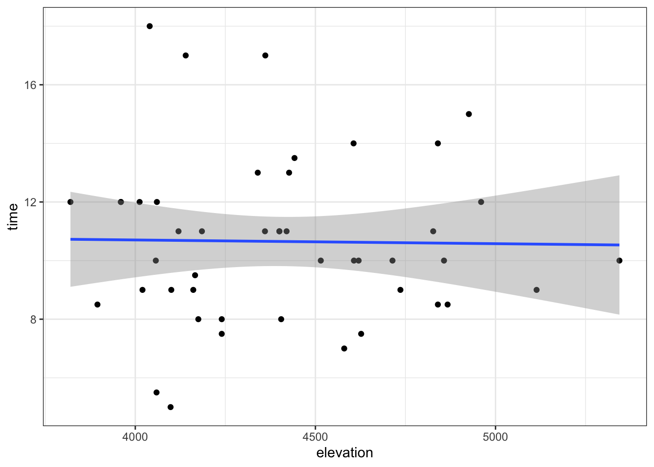

Exercise 8: time versus rating

# Visualize the relationship
ggplot(peaks, aes(y = time, x = rating)) + 
  geom_boxplot()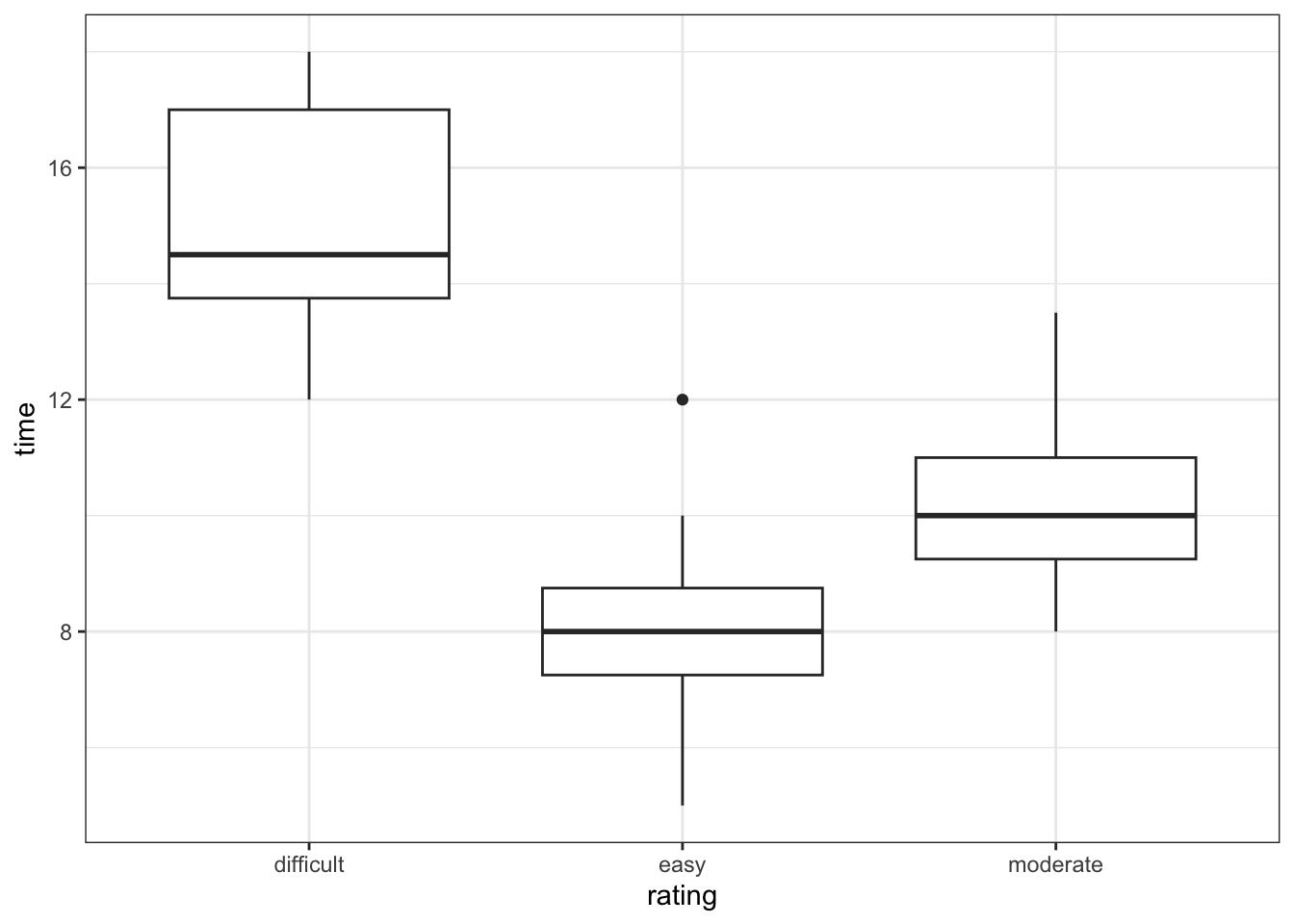


# Model the relationship
peaks_model_3 <- lm(time ~ rating, data = peaks)

# Obtain CIs for the model coefficients
confint(peaks_model_3)
##                    2.5 %    97.5 %
## (Intercept)    13.800649 16.199351
## ratingeasy     -8.576256 -5.423744
## ratingmoderate -5.921076 -3.190035

Part a

We’re 95% confident that…the average completion time of a moderate hike is between 3.19 and 5.92 hours less than that of a difficult hike

Part b

We’re 95% confident that…the average completion time of a difficult hike is between 13.8 and 16.2 hours.

Part c

Yes. The intervals for the moderate and easy rating coefficients both fall below 0, suggesting that completion times are significantly lower for moderate and easy hikes vs difficult hikes.

Exercise 9: Multiple logistic regression REVIEW

# NOTE: We'll take a sub-sample of 500 days for TEACHING PURPOSES ONLY
# In practice, we'd use all data in our sample :)
set.seed(155)
weather <- read_csv("https://mac-stat.github.io/data/weather_3_locations.csv") %>% 
  mutate(rain_tmrw = (raintomorrow == "Yes")) %>% 
  sample_n(size = 500, replace = FALSE)

# Build the sample model
weather_model_1 <- glm(rain_tmrw ~ location + humidity9am, data = weather, family = "binomial")
coef(summary(weather_model_1))
##                       Estimate  Std. Error   z value     Pr(>|z|)
## (Intercept)        -4.23087562 0.606988777 -6.970270 3.163334e-12
## locationUluru      -0.50422768 0.413866029 -1.218336 2.230965e-01
## locationWollongong  0.36535533 0.287787715  1.269531 2.042519e-01
## humidity9am         0.04001737 0.008110712  4.933891 8.060742e-07

# Exponentiate the coefficients
exp(-4.231)
## [1] 0.01453785
exp(-0.504)
## [1] 0.6041094
exp(0.040)
## [1] 1.040811

Part a

rain_tmrw is binary

Part b

On a day with 0 humidity at 9am in Hobart…

The odds of rain are 0.015.
The chance of rain is 1.5% as high as the chance of no rain.

Part c

When controlling for 9am humidity levels…

the odds of rain in Uluru are 60% as high as (hence 40% lower than) the odds in Hobart.

Part d

When controlling for location…

the odds of rain increase by 4% for every additional 1-percentage point increase in 9am humidity.

Exercise 10: Inference for logistic regression

Part a

confint(weather_model_1)
##                          2.5 %      97.5 %
## (Intercept)        -5.45851818 -3.07261857
## locationUluru      -1.35359732  0.28370308
## locationWollongong -0.19609539  0.93558070
## humidity9am         0.02437053  0.05626137

We do not have evidence that the chance of rain significantly differs in Uluru and Hobart when controlling for 9am humidity (i.e. when the 9am humidity is the same in both locations). 0 is in the interval!

Part b

exp(confint(weather_model_1))
##                          2.5 %     97.5 %
## (Intercept)        0.004259863 0.04629976
## locationUluru      0.258309366 1.32803856
## locationWollongong 0.821933830 2.54869305
## humidity9am        1.024669914 1.05787415

We do not have evidence that the chance of rain significantly differs in Uluru and Hobart when controlling for 9am humidity. 1 is in the interval

Part c

1. An odds ratio of 1 means that the odds for the 2 scenarios are not different. For example, if odds(rain | Uluru) / odds(rain | Hobart) = 1, then the odds of rain are the same in the 2 locations.

Exercise 11: Comparing models

Part a

Yes! The interval falls above 1.

Part b

weather_model_2 <- glm(rain_tmrw ~ location + humidity9am + humidity3pm, data = weather, family = "binomial")
exp(confint(weather_model_2))
##                          2.5 %     97.5 %
## (Intercept)        0.000851873 0.01438824
## locationUluru      0.785247399 6.16253858
## locationWollongong 0.341257492 1.26391403
## humidity9am        0.980908500 1.02314946
## humidity3pm        1.045270255 1.09967877

No! The CI includes 1.

Part c

When controlling for location, today’s 9am humidity includes “significant” information about the chance of rain. However, it doesn’t provide significant information on top of what’s provided by 3pm humidity. It’s likely the case that 9am and 3pm humidity are multicollinear, and 3pm humidity is the stronger predictor of tomorrow’s rain.