19  Hypothesis testing: discovery

Announcements etc

SETTLING IN

• Sit with your project group!
• Access the qmd here: “19-hypothesis-testing-discovery-notes.qmd”.
• Now is the final time to hand in Quiz 2 revisions for credit.

WRAPPING UP

Upcoming due dates:

• Thursday: CP 15
• Friday: PP 7
• Next week
  • Tuesday
    • Project Milestone 2 due
    • Project work day. Can’t be here? Consider Zooming in with your group. At minimum, coordinate a plan with them.
  • Thursday
    • No class. Thanksgiving break.

Learning goals

• Understand how standard errors and confidence intervals enable us to make statistical inferences
• Build intuition for concepts in hypothesis testing, including null values, test statistics, and p-values!

Warm-up

Let’s return to the fish dataset. Recall that rivers contain small concentrations of mercury which can accumulate in fish. Scientists studied this phenomenon among 171 largemouth bass in the Wacamaw and Lumber rivers of North Carolina, recording the following:

variable	meaning
Concen	Fish’s mercury concentration (in parts per million; ppm)
River	Lumber or Wacamaw
Length	Fish’s length (in centimeters)

# Load the data & packages
library(tidyverse)
fish <- read_csv("https://mac-stat.github.io/data/Mercury.csv")
head(fish)

GOAL

Use this sample data to make inferences about the relationship of mercury concentration (Concen) with the size of a fish, as measured by its Length. This relationship can be described by the population model:

\[ E[Concen | Length] = \beta_0 + \beta_1 Length \]

Our sample model is below:

\[ E[Concen | Length] = \hat{\beta}_0 + \hat{\beta}_1 Length = -1.132 + 0.058 Length \]

fish_mod_1 <- lm(Concen ~ Length, data = fish)
summary(fish_mod_1)

EXAMPLE 1: Review

Notation:

• \(\beta_1\) = the population parameter of interest whose “true” value is unknown
• \(\hat{\beta}_1\) = 0.058 is our sample estimate of \(\beta_1\)
• \(s.e.(\hat{\beta}_1)\) = 0.005 is the standard error of \(\hat{\beta}_1\)

1. Interpret \(\hat{\beta}_1\).

2. Using the 68-95-99.7 rule, construct an approximate 95% confidence interval for \(\beta_1\). That is, calculate an interval estimate of \(\beta_1\).

3. Compare your CI to an exact 95% CI:

___(___, level = 0.95)

4. Interpret the 95% CI in context.

EXAMPLE 2: Translating a hypothesis to notation

Our work above provides point and interval estimates of \(\beta_1\). But we also want to test hypotheses related to \(\beta_1\). Our fundamental hypothesis here is that, among the fish population, mercury levels are associated with fish length – there’s a relationship between the two. How can we state this hypothesis using notation?

• \(\beta_1 = 0\)
• \(\beta_1 \ne 0\)
• \(\hat{\beta}_1 = 0\)
• \(\hat{\beta}_1 \ne 0\)
• \(\beta_0 = 0\)
• \(\beta_0 \ne 0\)
• \(\hat{\beta}_0 = 0\)
• \(\hat{\beta}_0 \ne 0\)

NOTE: We’ll refer to 0 as the null value to which we’re comparing our population parameter of interest.

EXAMPLE 3: Evaluating a hypothesis using the CI

Since we don’t have access to the entire fish population, we must evaluate our hypothesis using our sample data. We have to ask: does our sample data provide enough evidence to support the hypothesis that, among the fish population, mercury levels are associated with fish length?

1. Explain why we can’t use our simple estimate \(\hat{\beta}_1\) to evaluate this hypothesis, but we can use the 95% CI for \(\beta_1\). (This is true in general, not just this fish example!)

2. So, does our 95% CI from Example 1 support the hypothesis that there’s a relationship between mercury levels and fish length? Explain.

3. Similarly, do the confidence bands below support the hypothesis?

fish %>% 
  ggplot(aes(y = Concen, x = Length)) + 
  geom_smooth(method = "lm") 

FORMAL HYPOTHESIS TESTS

Though CIs can help us evaluate hypotheses, hypothesis tests provide a more formal approach. The general idea:

1. Assume that the hypothesis is not true.
   
2. Determine what sample observations would be expected under this assumption.
   
3. Evaluate how compatible our observed sample data are with this assumption (are they consistent with what we’d expect?).

Or, in context:

1. Assume there were truly no association between mercury concentration and fish length, i.e. \(\beta_1 = 0\) (the “null value”).
2. Determine how our fish sample might have “behaved” if there were truly no association.
3. Evaluate how compatible our fish sample observations are with the null value (are they consistent with what we’d expect if there were no association?).

Exercises

NOTE

• The goal of these exercises is to explore concepts in hypothesis testing. There’s some new code that helps with this exploration, but the code is not the point!! Throughout, focus on the goal of the code and what its output tells us, NOT the details of the code.

• Our results will start to use more scientific notation. Examples:

  • 3e-02 = 0.03 (move the decimal 2 places to the left)
  • 3e02 = 300 (move the decimal 2 places to the right)
  • 4.12e-07 = 0.000000412 (move the decimal 7 places to the left)
  • 4.12e03 = 4120 (move the decimal 3 places to the right)
  • < 2e-16 = the result is less than 0.0000000000000002 (it’s really really small!)

Exercise 1: Simulating data under the null value

To begin testing our hypothesis that there is an association between mercury concentration and fish length (\(\beta_1 \ne 0\)), let’s explore how our sample data might behave IF in fact there were no association (\(\beta_1 = 0\)). We’ll first do this using simulation, and then through theory.

Part a

Read carefully:

• Suppose that when each individual fish in our sample was collected, the scientists wrote its Concen and Length on a piece of paper.

• They then ripped the paper in half, with the observed Concen on one half and the observed Length on the other.

• They then accidentally dropped the pieces of paper! In the resulting mess, they couldn’t tell which Length observation went with each Concen observation.

• To cover up their mistake, they just randomly matched up the Length and Concen pieces of paper. Essentially, in this shuffling process, the scientists broke the bond of the original Length and Concen pairs.

Question: Intuitively, if the researchers plotted the new pairs of Concen and Length values, what do you think their scatterplot would look like? What about their sample model?

Part b

We can simulate this idea in RStudio! Throughout, focus on concepts over code.

# First check out the first 6 fish
fish %>% 
  select(Concen, Length) %>% 
  head()

Now, randomly shuffle the Length values! That is, break the original Concen and Length pairs, and just randomly assign Length:

# Run this chunk a few times!!
# Shuffle the Length values
fish %>%
  select(Concen, Length) %>% 
  mutate(Length = sample(Length, size = length(Length), replace = FALSE)) %>% 
  head()

Let’s check out the sample models that arise from the shuffled Concen and Length pairs Summarize your observations! Was your intuition in Part a correct?

# Shuffle the Length values
# Run this chunk a few times!!
# Then plot the resulting sample data and model
fish %>% 
  select(Concen, Length) %>% 
  mutate(Length = sample(Length, size = length(Length), replace = FALSE)) %>% 
  ggplot(aes(x = Length, y = Concen)) + 
  geom_point() +
  geom_smooth(method = "lm")

Part c

These shuffled samples give us a sense of the sample models we’d expect IF \(\beta_1\) were actually 0, i.e. if there were no relationship between Concen and Length in the broader population of fish. To get a sense of the range of possible outcomes in this scenario, let’s simulate a bunch of these shuffled samples. Specifically, take 500 different shuffled samples and use each to estimate the model of Concen by Length (gray lines). Summarize your observations!! If there were truly no relationship between Concen and Length, how would we expect the sample data to behave?

set.seed(1)
shuffled_models <- mosaic::do(500)*(
  fish %>% 
  select(Concen, Length) %>% 
  sample_n(size = length(Length), replace = TRUE) %>% 
  mutate(Length = sample(Length, size = length(Length), replace = FALSE)) %>%
  with(lm(Concen ~ Length))
)
head(shuffled_models)

# Plot the 500 shuffled models
fish %>% 
  ggplot(aes(x = Length, y = Concen)) + 
  geom_abline(data = shuffled_models, 
              aes(intercept = Intercept, slope = Length), 
              color = "gray", size = 0.25) + 
  geom_smooth(method = "lm", se = FALSE, size = 0) # Ignore this line. It's a clunky workaround

Part d

Finally, focus on just the slope estimates \(\hat{\beta}_1\) behind the lines above. Summarize your observations!! If there were truly no relationship between Concen and Length, i.e. \(\beta_1\) were truly 0, how would we expect the sample slopes to behave?

shuffled_models %>% 
  ggplot(aes(x = Length)) + 
  geom_density()

Exercise 2: Comparing our sample results to the null value (intuition)

Now that we’ve simulated how sample data might behave if there were truly no relationship between Concen and Length (i.e. if \(\beta_1\) were 0), let’s consider the next important step in a hypothesis test:

Evaluate how compatible our observed sample data are with this assumption that \(\beta_1 = 0\)!

Part a

Let’s start with a visual assessment. Is our sample model (blue line) consistent / compatible with the “null models” simulated under the assumption the \(\beta_1 = 0\) (gray lines)?

fish %>% 
  ggplot(aes(x = Length, y = Concen)) + 
  geom_abline(data = shuffled_models, 
              aes(intercept = Intercept, slope = Length), 
              color = "gray", size = 0.25) + 
  geom_smooth(method = "lm", se = FALSE)

Part b

Consider another visual assessment, focusing just on the slopes of the lines in the plot above, i.e. our sample estimates \(\hat{\beta}_1\). Is our sample slope of \(\hat{\beta}_1 = 0.05813\) (blue line) consistent / compatible with the collection of slopes from the “null models” (density plot)?

shuffled_models %>% 
  ggplot(aes(x = Length)) + 
  geom_density() + 
  geom_vline(xintercept = 0.05813, color = "blue")

Part c

In Part b, you evaluated the compatibility of our sample slope \(\hat{\beta}_1 = 0.05813\) model with slopes of the “null models” using visual cues alone. But for a formal hypothesis test, we need some numerical measures of compatibility. Brainstorm some ideas!

Exercise 3: CLT

Now that we’ve built up some intuition using simulation, let’s formalize these concepts with some theory.

You shouldn’t be surprised to know that sampling distributions are at the heart of hypothesis testing! The distribution of slopes from our shuffled sample models uses simulation to approximate the sampling distribution of slope estimates \(\hat{\beta}_1\) we’d expect if the population slope \(\beta_1\) were actually 0 (the null value):

shuffled_models %>% 
  ggplot(aes(x = Length)) + 
  geom_density()

We can also approximate the sampling distribution using mathematical theory, specifically the Central Limit Theorem. If \(\beta_1\) were truly 0, then the distribution of possible sample estimates \(\hat{\beta}_1\) would be Normally distributed around 0:

\[ \hat{\beta}_1 \sim N(0, s.e.(\hat{\beta}_1)^2) \]

where in Example 1 we approximated the standard error to be 0.005. Thus a plot of the CLT is below. Confirm that this is similar to the simulated sampling distribution above:

# Don't worry about this code!!!
# Save your plot
clt_plot <- data.frame(x = 0 + c(-4:4)*0.005) %>% 
  mutate(y = dnorm(x, sd = 0.005)) %>% 
  ggplot(aes(x = x)) +
  stat_function(fun = dnorm, args = list(mean = 0, sd = 0.005)) +
  geom_segment(aes(x = x, xend = x, y = 0, yend = y), linetype = "dashed") + 
  scale_x_continuous(breaks = c(-4:4)*0.005) +
  labs(y = "density", x = "possible estimates IF the null value were true") 
  
clt_plot

Exercise 4: Comparing our sample results to the null value (test statistic)

Our sample slope estimate of \(\hat{\beta}_1 = 0.05813\) is shown on the sampling distribution of sample slopes \(\hat{\beta}_1\) that we’d expect if the population slope \(\beta_1\) were actually 0 (the null value):

clt_plot + 
  geom_vline(xintercept = 0.05813, color = "blue")

To measure how compatible (or incompatible) our estimate is with the null value, we can measure the distance between the two.

Part a

Our sample slope estimate of \(\hat{\beta}_1 = 0.05813\) is 0.05813 units (ppm/cm) from the null value of 0.

• In the context of this particular analysis, is that a big or a small number? How can you tell? That is, what info are you using to make this assessment?

• Would your answer be the same if you observed this estimate in another context?

Part b

In practice, we standardize our distance calculations so that they have the same meaning no matter the context of the analysis. We can do this by calculating a z-score:

\[ \frac{\hat{\beta}_1 - \text{null value}}{s.e.(\hat{\beta}_1)} = \text{ number of s.e. that $\hat{\beta}_1$ falls from the null value} \]

This is called the test statistic. Calculate and interpret the test statistic for our example.

Part c

Within rounding, the same test statistic appears in our model summary table! Where is it?!

coef(summary(fish_mod_1))

Part d

What can we conclude from your test statistic calculation and interpretation:

• Our sample data is not consistent with the null value of \(\beta_1 = 0\), i.e. the idea that there’s no significant association between mercury concentration and length.

• Our sample data is consistent with the null value of \(\beta_1 = 0\).

Exercise 5: Comparing our sample results to the null value (p-value)

Again, our sample slope estimate of \(\hat{\beta}_1 = 0.05813\) is shown on the sampling distribution of sample slopes \(\hat{\beta}_1\) that we’d expect if the population slope \(\beta_1\) were actually 0 (the null value):

clt_plot + 
  geom_vline(xintercept = 0.05813, color = "blue")

Part a

Another way to evaluate the compatibility of our estimate with the null value of \(\beta_1 = 0\) is to ask how likely we are to have gotten this estimate if the null value were indeed true! That is:

What’s the probability that we would have gotten a sample slope that’s at least 0.058 above or below 0 IF in fact there were no association between mercury concentration and length?

Equivalently, what’s the probability that we would have gotten a test statistic so far from 0 IF in fact \(\beta_1\) were 0?

Use the 68-95-99.7 Rule with the plot above to approximate the p-value:

• less than 0.003
• between 0.003 and 0.05
• between 0.05 and 0.32
• bigger than 0.32

Part b

The calculation above is called a p-value. A more accurate p-value is reported in the model summary table in the Pr(>|t|) column. What is it?

coef(summary(fish_mod_1))

Part c

How can we interpret the p-value? IMPORTANT: Think about the steps that went into calculating the p-value!!

• It’s very unlikely that we’d have observed such a steep increase in Concen with Length among our sample fish “by chance”, i.e. if in fact there were no relationship between mercury concentration and length in the broader fish population.

• Given what we observed in our sample data, it’s very unlikely that mercury concentration is associated with length.

• Given what we observed in our sample data, it’s very unlikely that mercury concentration and length are unrelated.

PAUSE: Check the solutions to this question! p-values are commonly misinterpreted.

Exercise 6: River test Part I

The fish in our sample come from two different rivers: Lumber and Wacamaw. Research question: Is there evidence that the mercury concentration in fish differs between the 2 rivers? To answer this question, we’ll control for fish Length – we don’t want to mistakenly detect a difference in mercury levels just because we happened to sample bigger fish in one river and smaller fish in the other. The relevant population model is:

\[ E[Concen | River, Length] = \beta_0 + \beta_1 RiverWacamaw + \beta_2 Length \]

Part a

To address the above research question, which model coefficient / population parameter is of primary interest: \(\beta_0\), \(\beta_1\), or \(\beta_2\)?

And what’s the null value of this coefficient? That is, what would this coefficient be if there were truly no difference in mercury concentration between the 2 rivers (when controlling for length)?

Part b

For the parameter of interest, obtain and report a sample estimate and its corresponding standard error:

fish_mod_2 <- lm(___, data = fish)

coef(summary(fish_mod_2))

Part c

Let’s use this data to evaluate our research question. To do so, remember the next step: Assume that the null value from Part a is correct and determine what sample estimates we would expect to get in this scenario.

Adjust the code below to sketch the appropriate sampling distribution. Represent our sample estimate by a blue line.

# Put OUR sample estimate here
# Round to 3 digits
est <- ___

# Put the corresponding standard error here
# Round to 3 digits
se <- ___

data.frame(x = 0 + c(-4:4)*se) %>% 
  mutate(y = dnorm(x, sd = se)) %>% 
  ggplot(aes(x = x)) +
  stat_function(fun = dnorm, args = list(mean = 0, sd = se)) +
  geom_segment(aes(x = x, xend = x, y = 0, yend = y), linetype = "dashed") + 
  scale_x_continuous(breaks = c(-4:4)*se) + 
  geom_vline(xintercept = est, color = "blue") +
  labs(y = "density", x = "possible estimates IF the null value were true") 

Exercise 7: River test Part II

Remember the next step: We must evaluate how compatible our sample estimate is with the null value. We’ll take 3 approaches: using a visual assessment, test statistic, and p-value.

Part a

Visually, in Part c of the previous exercise, does our sample estimate seem compatible with the null value? Mainly, is our estimate consistent with what we’d expect to observe if there were truly no difference in the mercury concentration between the 2 rivers (when controlling for fish length)?

Part b

• Obtain the test statistic from the model summary table below.
• Show how this was calculated from the sample estimate and its standard error.
• Interpret the test statistic.

coef(summary(fish_mod_2))

Part c

Recall that the p-value calculates the probability that we would have gotten a sample estimate that’s as far from the null value as ours (hence a test statistic that’s as far from 0), IF in fact the null value were correct (i.e. there were actually no difference in mercury concentration by river when controlling for length). First, use the 68-95-99.7 Rule with the plot in Part c of the previous exercise to approximate the p-value:

• less than 0.003
• between 0.003 and 0.05
• between 0.05 and 0.32
• bigger than 0.32

Next, obtain and report the exact p-value from the model summary table.

coef(summary(fish_mod_2))

Part d

Do your test statistic and p-value indicate that your estimate is or is not compatible with the null value? Explain.

Part e

Putting this all together, what do you conclude? When controlling for length…

• we have evidence of a statistically significant difference in mercury concentration by river.
• we do not have sufficient evidence to conclude that there’s a statistically significant difference in mercury concentration by river.

Exercise 8: River CI

Part a

Finally, check out a 95% CI for the population parameter of interest in our river analysis:

confint(fish_mod_2)

What do you conclude from this CI? When controlling for length…

• we have evidence of a statistically significant difference in mercury concentration by river.
• we do not have sufficient evidence to conclude that there’s a statistically significant difference in mercury concentration by river.

Part b

Your conclusions from the hypothesis test (test statistic and p-value) should agree with those from your CI! If this is not the case, review your work.

Done?

Work on Project Milestone 2 with your group!! Things to think about:

• Check out the directions on Moodle.
• Narrow down your research topic.
• Start thinking about:
  • what you observe in your sample
  • what you can infer about the broader population
  • WHY this might be – what explains the patterns you’ve observed

Solutions

# Load the data & packages
library(tidyverse)
fish <- read_csv("https://mac-stat.github.io/data/Mercury.csv")
head(fish)
## # A tibble: 6 × 5
##   River  Station Length Weight Concen
##   <chr>    <dbl>  <dbl>  <dbl>  <dbl>
## 1 Lumber       0   47     1616   1.6 
## 2 Lumber       0   48.7   1862   1.5 
## 3 Lumber       0   55.7   2855   1.7 
## 4 Lumber       0   45.2   1199   0.73
## 5 Lumber       0   44.7   1320   0.56
## 6 Lumber       0   43.8   1225   0.51

fish_mod_1 <- lm(Concen ~ Length, data = fish)
summary(fish_mod_1)
## 
## Call:
## lm(formula = Concen ~ Length, data = fish)
## 
## Residuals:
##     Min      1Q  Median      3Q     Max 
## -1.1499 -0.3436 -0.1022  0.3123  1.9100 
## 
## Coefficients:
##              Estimate Std. Error t value Pr(>|t|)    
## (Intercept) -1.131645   0.213615  -5.298 3.62e-07 ***
## Length       0.058127   0.005228  11.119  < 2e-16 ***
## ---
## Signif. codes:  0 '***' 0.001 '**' 0.01 '*' 0.05 '.' 0.1 ' ' 1
## 
## Residual standard error: 0.5805 on 169 degrees of freedom
## Multiple R-squared:  0.4225, Adjusted R-squared:  0.4191 
## F-statistic: 123.6 on 1 and 169 DF,  p-value: < 2.2e-16

EXAMPLE 1: Review

1. We estimate that for every 1cm increase in length, the expected mercury concentration increases by 0.058ppm.

2. \(0.058 \pm 2*0.005 = (0.058 - 0.010, 0.058 + 0.010) = (0.048, 0.068)\)

3. .

confint(fish_mod_1, level = 0.95)
##                   2.5 %      97.5 %
## (Intercept) -1.55334248 -0.70994835
## Length       0.04780769  0.06844728

4. We’re 95% confident that for every 1cm increase in length, the expected mercury concentration increases by somewhere between 0.048ppm and 0.068ppm.

EXAMPLE 2: Translating a hypothesis to notation

• \(\beta_1 \ne 0\)

EXAMPLE 3: Evaluating a hypothesis using the CI

1. The simple estimate \(\hat{\beta}_1\) has error that we need to account for when making inferences about the population. The CI accounts for this error!

2. Yes, the interval doesn’t include 0. Thus 0 is not a plausible value for \(\beta_1\).

3. Yes, a 0-slope line cannot be drawn within these confidence bands.

fish %>% 
  ggplot(aes(y = Concen, x = Length)) + 
  geom_smooth(method = "lm")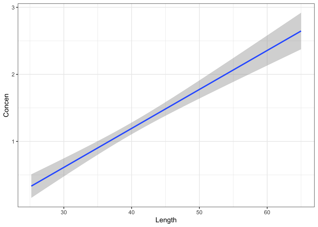 

Exercise 1: Simulating data under the null value

Part a

Intuition.

Part b

# First check out the first 6 fish
fish %>% 
  select(Concen, Length) %>% 
  head()
## # A tibble: 6 × 2
##   Concen Length
##    <dbl>  <dbl>
## 1   1.6    47  
## 2   1.5    48.7
## 3   1.7    55.7
## 4   0.73   45.2
## 5   0.56   44.7
## 6   0.51   43.8

# Run this chunk a few times!!
# Shuffle the Length values
fish %>%
  select(Concen, Length) %>% 
  mutate(Length = sample(Length, size = length(Length), replace = FALSE)) %>% 
  head()
## # A tibble: 6 × 2
##   Concen Length
##    <dbl>  <dbl>
## 1   1.6    48.1
## 2   1.5    30  
## 3   1.7    30  
## 4   0.73   28.5
## 5   0.56   44.7
## 6   0.51   47.2

# Shuffle the Length values
# Run this chunk a few times!!
# Then plot the resulting sample data and model
fish %>% 
  select(Concen, Length) %>% 
  mutate(Length = sample(Length, size = length(Length), replace = FALSE)) %>% 
  ggplot(aes(x = Length, y = Concen)) + 
  geom_point() +
  geom_smooth(method = "lm")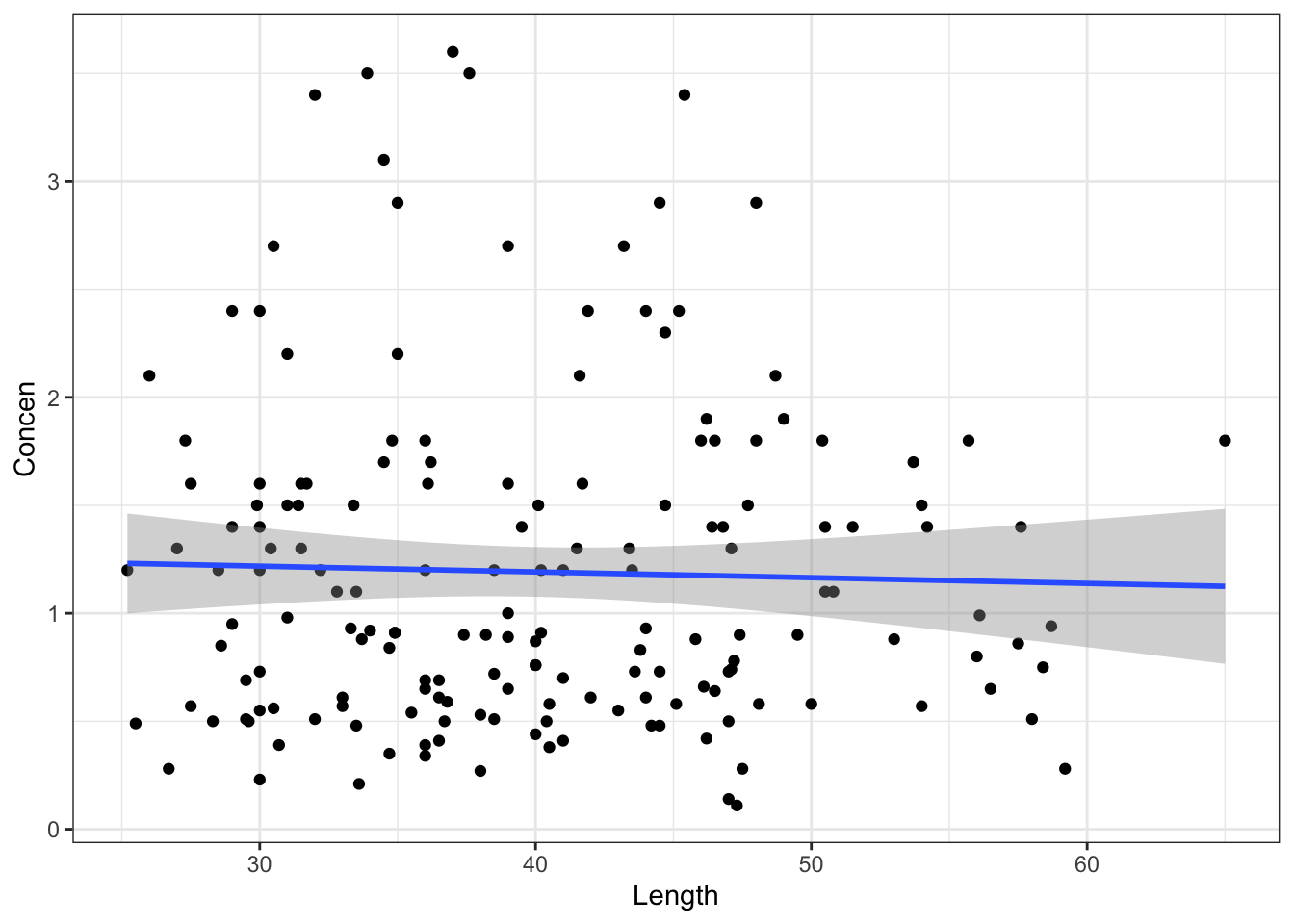

Part c

If there were truly no relationship between Concen and Length, we’d expect the sample model to have a slope near to (but not exactly) 0.

set.seed(1)
shuffled_models <- mosaic::do(500)*(
  fish %>% 
  select(Concen, Length) %>% 
  sample_n(size = length(Length), replace = TRUE) %>% 
  mutate(Length = sample(Length, size = length(Length), replace = FALSE)) %>%
  with(lm(Concen ~ Length))
)
head(shuffled_models)
##   Intercept        Length     sigma    r.squared           F numdf dendf .row
## 1 0.7994259  0.0075368727 0.6765800 7.371664e-03 1.255063194     1   169    1
## 2 0.9584317  0.0037391031 0.7811844 2.031882e-03 0.344087261     1   169    1
## 3 0.8270447  0.0089664603 0.7691294 9.240981e-03 1.576292349     1   169    1
## 4 0.7629911  0.0118477349 0.8498595 1.539909e-02 2.643148655     1   169    1
## 5 1.0765620 -0.0004547678 0.6746811 2.931604e-05 0.004954555     1   169    1
## 6 0.5069886  0.0188557911 0.8317681 3.879420e-02 6.820829143     1   169    1
##   .index
## 1      1
## 2      2
## 3      3
## 4      4
## 5      5
## 6      6

fish %>% 
  ggplot(aes(x = Length, y = Concen)) + 
  geom_abline(data = shuffled_models, 
              aes(intercept = Intercept, slope = Length), 
              color = "gray", size = 0.25) + 
  geom_smooth(method = "lm", se = FALSE, size = 0) # Ignore this line. It's a clunky workaround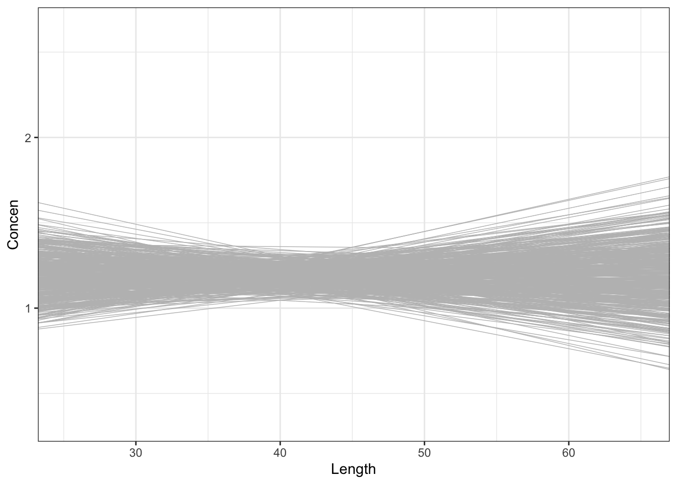

Part d

We’d expect slopes to be Normally distributed around 0 (the null value).

shuffled_models %>% 
  ggplot(aes(x = Length)) + 
  geom_density()

Exercise 2: Comparing our sample results to the null value (intuition)

Part a

No! Its slope is much bigger than for the sample models simulated using the null value!

fish %>% 
  ggplot(aes(x = Length, y = Concen)) + 
  geom_abline(data = shuffled_models, 
              aes(intercept = Intercept, slope = Length), 
              color = "gray", size = 0.25) + 
  geom_smooth(method = "lm", se = FALSE)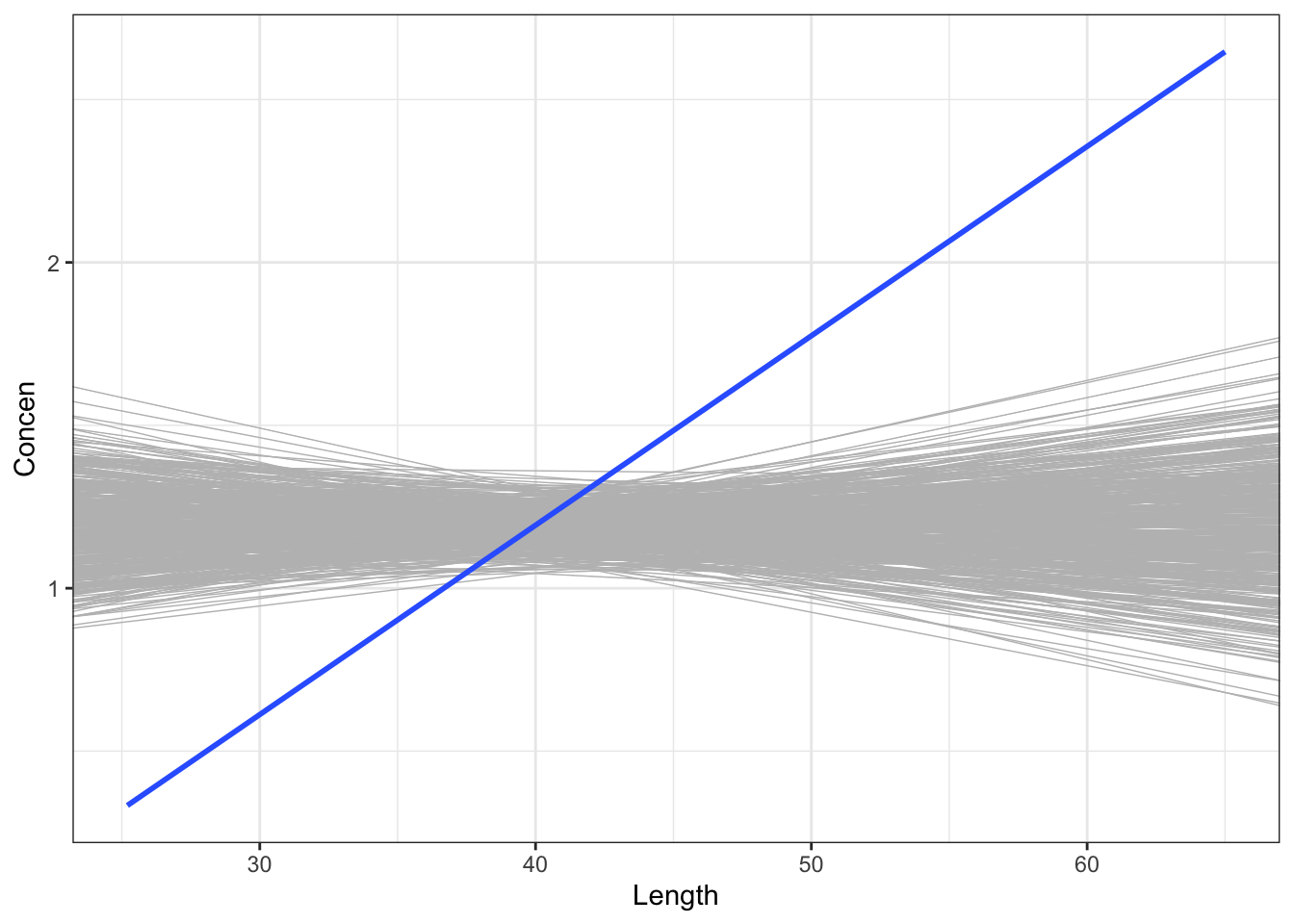

Part b

No! Our slope is much bigger than for the sample models simulated using the null value!

shuffled_models %>% 
  ggplot(aes(x = Length)) + 
  geom_density() + 
  geom_vline(xintercept = 0.05813, color = "blue")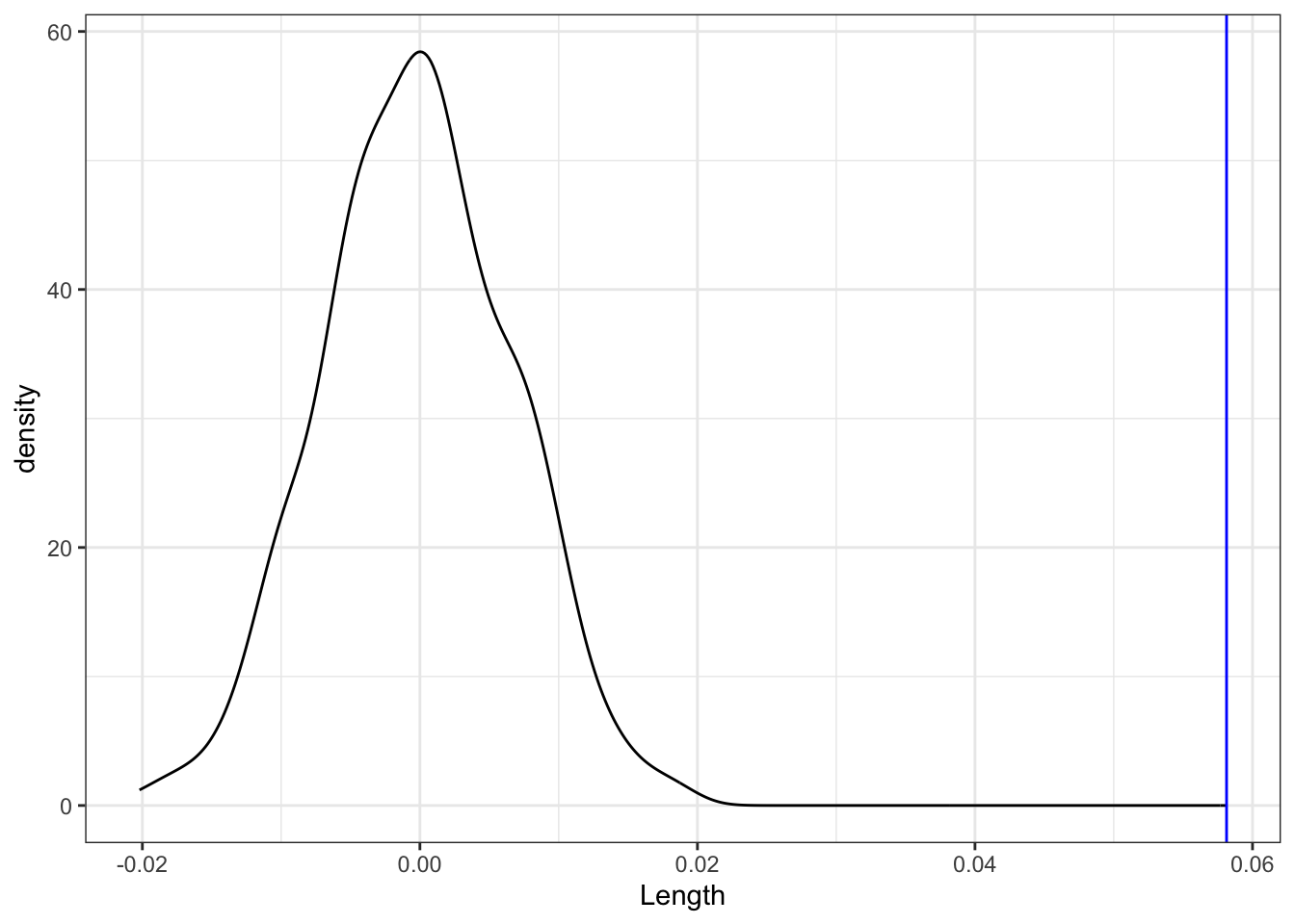

Part c

Will vary.

Exercise 3: CLT

The simulated and CLT / theory-informed sampling distributions are similar!

shuffled_models %>% 
  ggplot(aes(x = Length)) + 
  geom_density()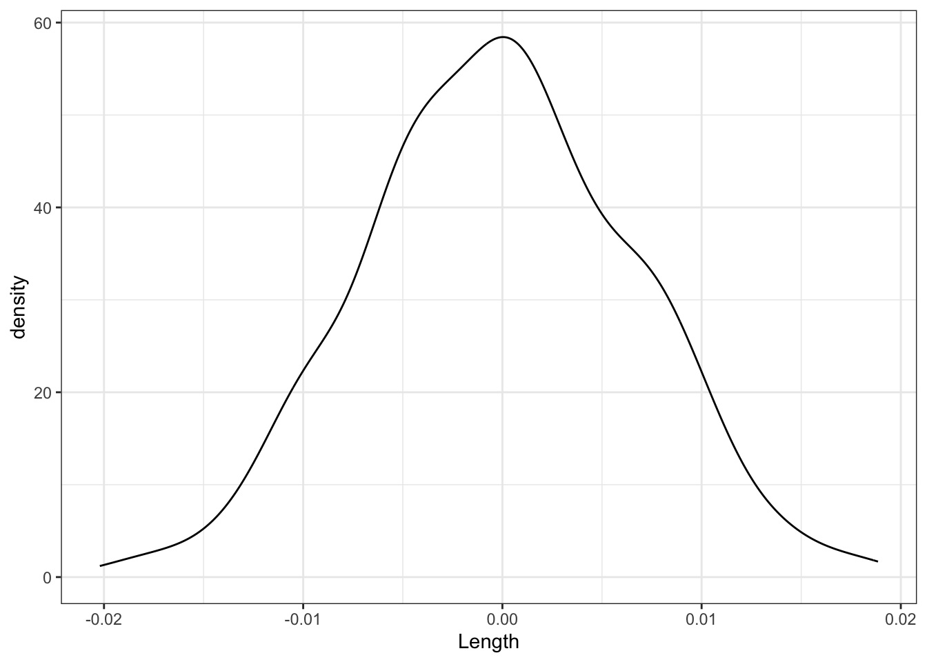

clt_plot <- data.frame(x = 0 + c(-4:4)*0.005) %>% 
  mutate(y = dnorm(x, sd = 0.005)) %>% 
  ggplot(aes(x = x)) +
  stat_function(fun = dnorm, args = list(mean = 0, sd = 0.005)) +
  geom_segment(aes(x = x, xend = x, y = 0, yend = y), linetype = "dashed") + 
  scale_x_continuous(breaks = c(-4:4)*0.005) +
  labs(y = "density", x = "possible estimates IF the null value were true") 
  
clt_plot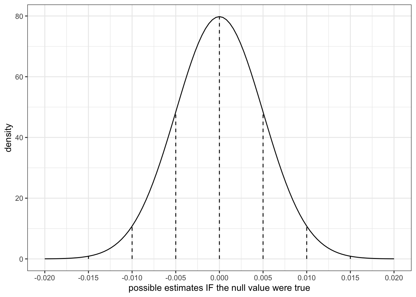

Exercise 4: Comparing our sample results to the null value (test statistic)

clt_plot + 
  geom_vline(xintercept = 0.05813, color = "blue")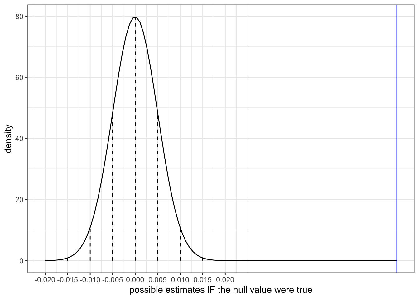

Part a

• This seems pretty big relative to the standard error of 0.005.
• In another context, 0.058127 might be a small number, depending on the units!

Part b

Our sample slope of 0.058 falls more than 11 standard errors above the null value of 0. That’s far!!!

(0.058127 - 0) / 0.005228
## [1] 11.1184

Part c

In the t value column:

coef(summary(fish_mod_1))
##                Estimate  Std. Error   t value     Pr(>|t|)
## (Intercept) -1.13164542 0.213614796 -5.297598 3.617750e-07
## Length       0.05812749 0.005227593 11.119359 6.641225e-22

Part d

• Our sample data is not consistent with the null value of \(\beta_1 = 0\), i.e. the idea that there’s no significant association between mercury concentration and length.

Exercise 5: Comparing our sample results to the null value (p-value)

clt_plot + 
  geom_vline(xintercept = 0.05813, color = "blue")

Part a

Our estimate is more than 3 s.e. away from 0. Since 99.7% of estimates fall within 3 s.e. the probability of this happening is…

• less than 0.003 (1 - 0.997)

Part b

< 2e-16 (which is very very close to 0)

coef(summary(fish_mod_1))
##                Estimate  Std. Error   t value     Pr(>|t|)
## (Intercept) -1.13164542 0.213614796 -5.297598 3.617750e-07
## Length       0.05812749 0.005227593 11.119359 6.641225e-22

Part c

• It’s very unlikely that we’d have observed such a steep increase in Concen with Length among our sample fish “by chance”, i.e. if in fact there were no relationship between mercury concentration and length in the broader fish population.

Exercise 6: River test Part I

Part a

\(\beta_1\), the RiverWacamaw coefficient

The null value is \(\beta_1 = 0\)

Part b

\(\hat{\beta}_1 = 0.142\) with a standard error of 0.089:

fish_mod_2 <- lm(Concen ~ River + Length, data = fish)

coef(summary(fish_mod_2))
##                 Estimate  Std. Error   t value     Pr(>|t|)
## (Intercept)  -1.19422929 0.216287220 -5.521497 1.255595e-07
## RiverWacamaw  0.14202739 0.089496454  1.586961 1.144018e-01
## Length        0.05765684 0.005212709 11.060821 1.033822e-21

Part c

# Put OUR sample estimate here
# Round to 3 digits
est <- 0.142

# Put the corresponding standard error here
# Round to 3 digits
se <- 0.089

data.frame(x = 0 + c(-4:4)*se) %>% 
  mutate(y = dnorm(x, sd = se)) %>% 
  ggplot(aes(x = x)) +
  stat_function(fun = dnorm, args = list(mean = 0, sd = se)) +
  geom_segment(aes(x = x, xend = x, y = 0, yend = y), linetype = "dashed") + 
  scale_x_continuous(breaks = c(-4:4)*se) + 
  geom_vline(xintercept = est, color = "blue") +
  labs(y = "density", x = "possible estimates IF the null value were true")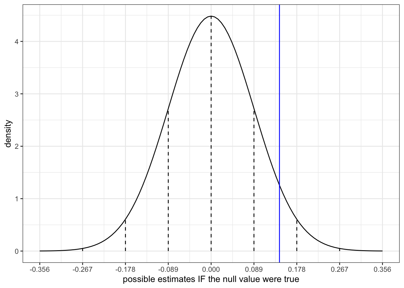 

Exercise 7: River test Part II

Part a

Yes! Our estimate is relatively close to 0 on this scale (within 2 s.e.).

Part b

Our estimate of \(\beta_1\), 0.142, falls only 1.59 s.e. from 0:

(0.142 - 0) / 0.089
## [1] 1.595506
coef(summary(fish_mod_2))
##                 Estimate  Std. Error   t value     Pr(>|t|)
## (Intercept)  -1.19422929 0.216287220 -5.521497 1.255595e-07
## RiverWacamaw  0.14202739 0.089496454  1.586961 1.144018e-01
## Length        0.05765684 0.005212709 11.060821 1.033822e-21

Part c

Our estimate is somewhere between 1 and 2 s.e. from 0:

• between 0.05 and 0.32

An exact p-value is 0.114:

coef(summary(fish_mod_2))
##                 Estimate  Std. Error   t value     Pr(>|t|)
## (Intercept)  -1.19422929 0.216287220 -5.521497 1.255595e-07
## RiverWacamaw  0.14202739 0.089496454  1.586961 1.144018e-01
## Length        0.05765684 0.005212709 11.060821 1.033822e-21

Part d

It is. It is not very far from 0 (when considering s.e.) and would not be unlikely to observe if the null value were true.

Part e

When controlling for length…

• we do not have sufficient evidence to conclude that there’s a statistically significant difference in mercury concentration by river.

Exercise 8: River CI

Part a

confint(fish_mod_2)
##                    2.5 %     97.5 %
## (Intercept)  -1.62122031 -0.7672383
## RiverWacamaw -0.03465518  0.3187100
## Length        0.04736599  0.0679477

Since 0 IS in the CI: When controlling for length…we do not have sufficient evidence to conclude that there’s a statistically significant difference in mercury concentration by river.