21 Bivariate Normal & Correlation
READING
For more on this topic, read B & H Chapter 7.5.
21.1 Discussion
GOAL
We’ve been exploring different multivariate probability models. One of the most common is the multivariate Normal model. Today, we’ll focus on the simplified bivariate setting.
BIVARIATE NORMAL MODEL
Suppose \(X\) and \(Y\) are (jointly) bivariate Normal with 5 parameters, \((\mu_X, \mu_Y, \sigma_X, \sigma_Y, \rho)\) where \(\rho\) is the Greek letter “rho”. The model is represented by the following notation:
\[\left(\begin{array}{c} X \\ Y \end{array}\right) \sim N \left(\left(\begin{array}{c} \mu_X \\ \mu_Y \end{array}\right), \; \left(\begin{array}{cc} \sigma^2_X & \rho \sigma_X \sigma_Y\\ \rho \sigma_X \sigma_Y & \sigma^2_Y \end{array}\right) \right)\]
and is specified by the bivariate pdf with support \(x,y \in (-\infty, \infty)\): \[ \begin{split} f_{X,Y}(x,y) & = \frac{1}{\sigma_X \sigma_Y \sqrt{1 - \rho^2}\left(\sqrt{2 \pi}\right)^2} \\ & \cdot \exp \left\lbrace -\frac{1}{2(1-\rho^2)}\left[ \left(\frac{x-\mu_X}{\sigma_X}\right)^2 + \left(\frac{y-\mu_Y}{\sigma_Y}\right)^2 - 2\rho\left(\frac{x-\mu_X}{\sigma_X}\right)\left(\frac{y-\mu_Y}{\sigma_Y}\right) \right]\right\rbrace \\ \end{split} \]
WARM-UP: SIMULATION
To get some intuition for this model, let’s start with a simulation. First, load the following packages (you might first have to install these):
Next, copy and paste the following function which will simulate 10,000 draws from a bivariate Normal model:
normal_sim <- function(mean_x, mean_y, sd_x, sd_y, rho){
    # Bivariate trend
    mean_xy <- c(mean_x, mean_y)

    # Bivariate deviation from trend
    cov <- rho * sd_x * sd_y
    cov_mat <- matrix(c(sd_x^2, cov, cov, sd_y^2), nrow = 2)

    # Simulate a random sample of 10000 observations
    bivariate_data <- data.frame(rmvnorm(n = 10000, mean = mean_xy, sigma = cov_mat))
    names(bivariate_data) <- c("x", "y")

    # Return the data
    bivariate_data
}
The remainder of the code is provided below if you’re curious.
Example 1
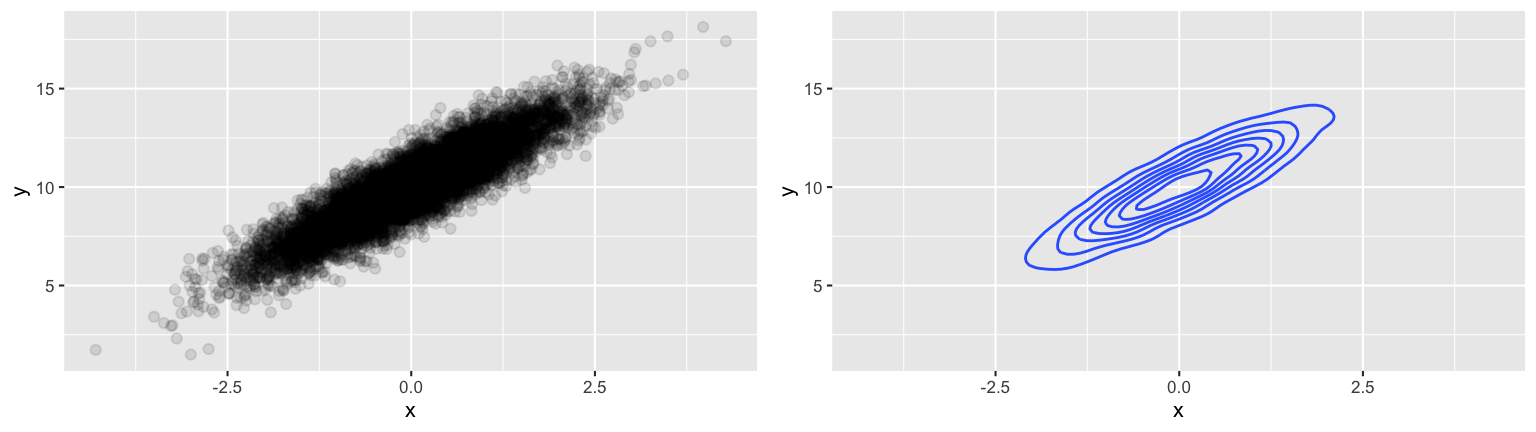
Simulate 10,000 draws from the bivariate Normal model with \(\mu_X = 0\), \(\mu_Y = 10\), \(\sigma_X = 1\), \(\sigma_Y = 2\), \(\rho = 0.95\):
\[\left(\begin{array}{c} X \\ Y \end{array}\right) \sim N \left(\left(\begin{array}{c} 0 \\ 10 \end{array}\right), \; \left(\begin{array}{cc} 1 & 1.9\\ 1.9 & 2^2 \end{array}\right) \right)\] and check out a scatterplot and contour plot of the simulated \((X,Y)\) pairs. Based on these plots, try to identify how the 5 parameters (\(\mu_X,\mu_Y,\sigma_X,\sigma_Y,\rho)\) are exhibited in the simulated data. NOTE: \(\rho\) is a new concept. If you get stuck on that parameter, just move on and it will soon be clear!
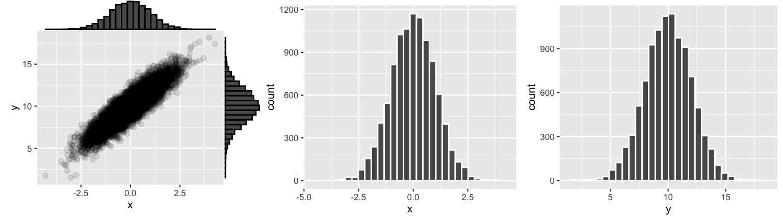
Example 2: Marginal behavior
We simulated 10,000 \((X,Y)\) pairs from the bivariate Normal model. Next, examine visualizations of the marginal behaviors of \(X\) and \(Y\). Based on these plots and your intuition alone, try to identify the marginal models of \(X\) and \(Y\).
\[\begin{split} X & \sim \hspace{2.5in}\\ Y & \sim \hspace{2.5in}\\ \end{split}\]
THINK: How are the parameters of the marginal model defined by the parameters of the bivariate model (\(\mu_X,\mu_Y,\sigma_X,\sigma_Y,\rho\))?
Code
Example 3: Conditional behavior
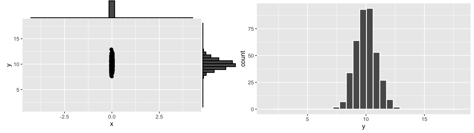
Suppose we know that \(X = 0\). What does this tell us about \(Y\)? In order to examine the conditional model of \(Y\) given the data that \(X=0\), we can examine the simulated data with \(X\) values near 0. (Why not just look at the simulated data where \(X\) is exactly 0???)
head(sim_data, 3)
##             x         y
## 1 -0.14772007  9.884809
## 2  0.08645436 11.510782
## 3  0.22048604 13.168393

# Conditional: X approx 0
cond_data_0 <- sim_data %>%
  filter(x > -0.05, x < 0.05)
dim(cond_data_0)
## [1] 385   2
Next, check out the conditional behavior of \(Y\) given \(X \approx 0\):
Similarly, check out the conditional behavior of \(Y\) when \(X \approx 1\):
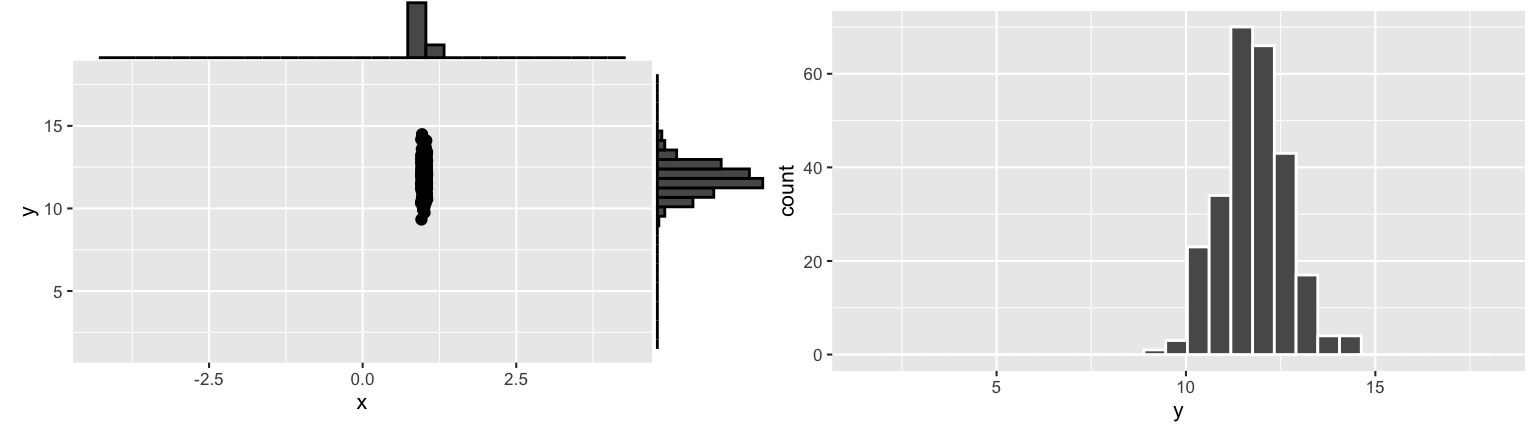
Based on these plots and your intuition alone, try to identify the following conditional models of \(Y\):
\[\begin{split} Y|(X=0) & \sim \hspace{2.5in}\\ Y|(X=1) & \sim \hspace{2.5in}\\ \end{split}\]
THINK:
- Do these two conditional models have the same expected values? The same variances?
- How are the parameters of the conditional model defined by the parameters of the bivariate model (\(\mu_X,\mu_Y,\sigma_X,\sigma_Y,\rho\))? This is a bit tougher than in the marginal case!!
# Within the scatterplot
p <- ggplot(cond_data_0, aes(x, y)) +
    geom_point() +
    lims(x = range(sim_data$x), y = range(sim_data$y))
ggExtra::ggMarginal(p, type = "histogram")

# Y alone
ggplot(cond_data_0, aes(x = y)) +
    geom_histogram(color = "white") +
    lims(x = range(sim_data$y))

# Conditional: X approx 1
cond_data_1 <- sim_data %>%
    filter(x > 0.95, x < 1.05)

p <- ggplot(cond_data_1, aes(x, y)) +
    geom_point() +
    lims(x = range(sim_data$x), y = range(sim_data$y))
ggExtra::ggMarginal(p, type = "histogram")

ggplot(cond_data_1, aes(x = y)) +
    geom_histogram(color = "white") +
    lims(x = range(sim_data$y))
Example 4: Play around with \(\rho\)
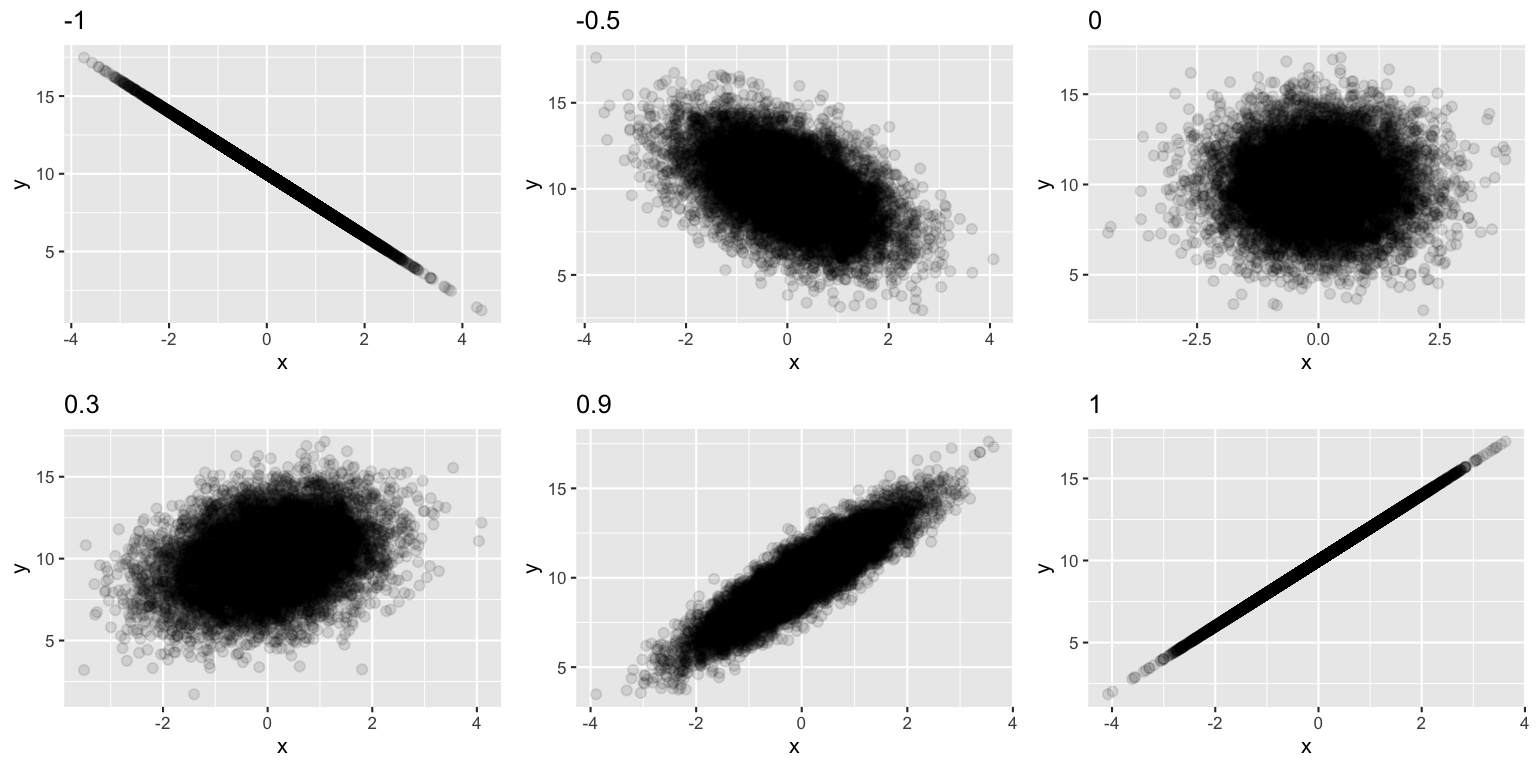
\(\rho\) is a new type of model feature – a correlation. Use the plots below to identify which \(\rho\) values that would produce the following features:
- a strong negative association between \(X\) and \(Y\);
- a moderate positive association between \(X\) and \(Y\);
- a very weak to no association between \(X\) and \(Y\).
rho_plot <- function(my_rho){
  sim_data <- normal_sim(mean_x = 0, mean_y = 10, sd_x = 1, sd_y = 2, rho = my_rho)
  ggplot(sim_data, aes(x, y)) +
    geom_point(alpha = 0.1) +
    labs(title = paste(my_rho))
}

set.seed(354)
g1 <- rho_plot(-1)
g2 <- rho_plot(-0.5)
g3 <- rho_plot(0)
g4 <- rho_plot(0.3)
g5 <- rho_plot(0.9)
g6 <- rho_plot(1)

grid.arrange(g1,g2,g3,g4,g5,g6,ncol=3)
BIVARIATE NORMAL
Suppose \(X\) and \(Y\) are (jointly) bivariate Normal with 5 parameters:
- expected values \(E(X)=\mu_X\) and \(E(Y) = \mu_Y\)
- standard deviations \(SD(X) = \sigma_X\) and \(SD(Y) = \sigma_Y\)
- correlation \(Cor(X,Y)=\rho\) (“rho”)
The model is represented by the following notation:
\[\left(\begin{array}{c} X \\ Y \end{array}\right) \sim N \left(\left(\begin{array}{c} \mu_X \\ \mu_Y \end{array}\right), \; \left(\begin{array}{cc} \sigma^2_X & \rho \sigma_X \sigma_Y\\ \rho \sigma_X \sigma_Y & \sigma^2_Y \end{array}\right) \right)\]
and is specified by the following joint pdf which has support \(x,y \in (-\infty, \infty)\): \[ \begin{split} f_{X,Y}(x,y) & = \frac{1}{\sigma_X \sigma_Y \sqrt{1 - \rho^2}\left(\sqrt{2 \pi}\right)^2} \\ & \cdot \exp \left\lbrace -\frac{1}{2(1-\rho^2)}\left[ \left(\frac{x-\mu_X}{\sigma_X}\right)^2 + \left(\frac{y-\mu_Y}{\sigma_Y}\right)^2 - 2\rho\left(\frac{x-\mu_X}{\sigma_X}\right)\left(\frac{y-\mu_Y}{\sigma_Y}\right) \right]\right\rbrace \\ \end{split} \]
EXAMPLES
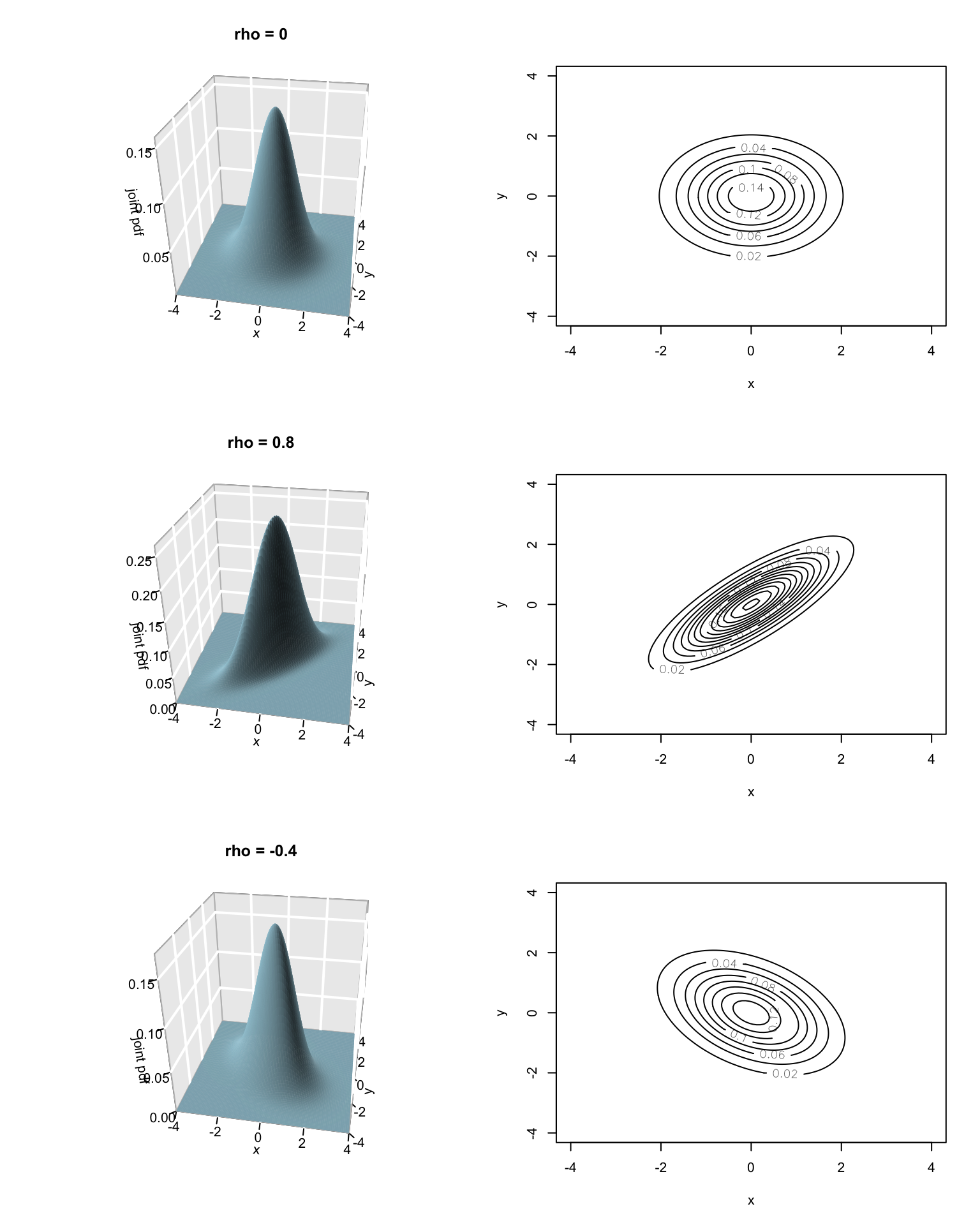
For example, each of the following models have the following form with different \(\rho\):
\[\left(\begin{array}{c} X \\ Y \end{array}\right) \sim N \left(\left(\begin{array}{c} 0 \\ 0 \end{array}\right), \; \left(\begin{array}{cc} 1 & \rho \\ \rho & 1 \end{array}\right) \right)\]
CORRELATION & COVARIANCE
Correlation \(Cor(X,Y)=\rho \in [-1,1]\) is a measure of the strength and direction of a linear relationship:
\(\rho \approx -1\) indicates a strong negative correlation
\(\rho \approx 0\) indicates a weak correlation
\(\rho \approx 1\) indicates a strong positive correlation
We can calculate the correlation between two RVs \(X\) and \(Y\) by
\[\rho = \frac{Cov(X,Y)}{SD(X)SD(Y)} = \frac{E((X-E(X))(Y - E(Y)))}{SD(X)SD(Y)}\;.\]
Where \(Cov(X,Y) = E((X-E(X))(Y - E(Y)))\) is the covariance of \(X\) and \(Y\). It measures how \(X\) and \(Y\) co-vary.
Details
\(Cov(X,Y) = E((X-E(X))(Y - E(Y))) > 0\)
Covariance is positive when greater values of \(X\) (relative to \(E(X)\)) typically occur with greater values of \(Y\) (relative to \(E(Y)\)) and smaller values of \(X\) typically occur with smaller values of \(Y\)\(Cov(X,Y) = E((X-E(X))(Y - E(Y))) < 0\)
Covariance is negative when greater values of \(X\) (relative to \(E(X)\)) typically occur with smaller values of \(Y\) (relative to \(E(Y)\)) and smaller values of \(X\) typically occur with greater values of \(Y\)Dividing \(Cov(X,Y)\) by \(SD(X)SD(Y)\) normalizes the measure of co-variability relative to the magnitude of variability in \(X\) and \(Y\)
Marginal vs (joint) Bivariate vs Conditional Normality
If \(X, Y\) are jointly Normal,
\[\left(\begin{array}{c} X \\ Y \end{array}\right) \sim N \left(\left(\begin{array}{c} \mu_X \\ \mu_Y \end{array}\right), \; \left(\begin{array}{cc} \sigma^2_X & \rho \sigma_X \sigma_Y\\ \rho \sigma_X \sigma_Y & \sigma^2_Y \end{array}\right) \right) \;\; \]
Then they’re both marginally Normal:
\[\begin{split} X & \sim N \left(\mu_X, \sigma_X^2\right) \\ Y & \sim N \left(\mu_Y, \sigma_Y^2\right) \\ \end{split}\]
And conditionally Normal: \[ Y|(X=x) \sim N \left(\mu_Y + \frac{\sigma_Y}{\sigma_X} \rho (x-\mu_X), \; (1-\rho^2)\sigma_Y^2\right) \]
NOTE: We could set up formulas that could be used to prove these features (if we had time and patience).
21.2 Exercises
Directions
To check your work, solutions are provided for each exercise in the online course manual. You can also see these exercises worked through on the video.
Unless told to “prove” something, you can and should utilize any features of the univariate, bivariate, and conditional Normal models that you’ve learned today and previously.
For quick reference, the properties of a univariate Normal model are summarized below. If
\[X \sim N(\mu, \sigma^2)\] Then \[\begin{split} f_X(x) & = \frac{1}{\sqrt{2 \pi \sigma^2}} e^{-\frac{1}{2}\left(\frac{x-\mu}{\sigma} \right)^2} = \frac{1}{\sqrt{2 \pi \sigma^2}} \exp\left\lbrace -\frac{1}{2}\left(\frac{x-\mu}{\sigma} \right)^2\right\rbrace \;\;\; \text{ for } x \in (-\infty,\infty) \\ M_X(t) & = \exp \left\lbrace \mu t + \frac{1}{2}\sigma^2 t^2\right\rbrace \\ E(X) & = \mu \\ Var(X) & = \sigma^2 \\ SD(X) & = \sigma \\ \end{split}\]
The Story
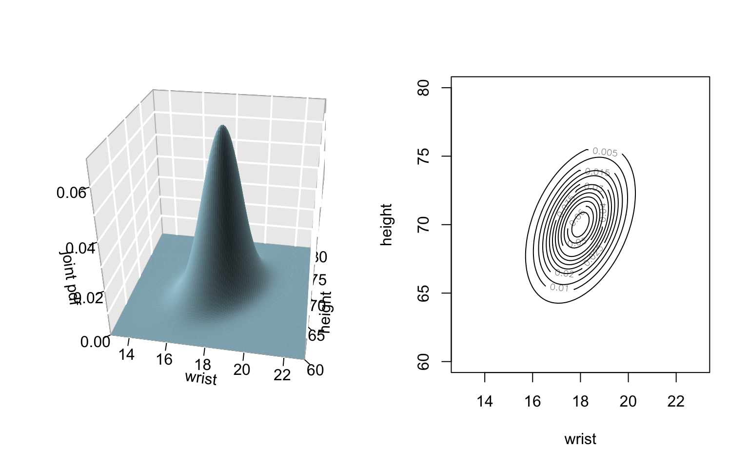
In this case study we’ll explore the bivariate Normal and correlation concepts in an intuitive setting: the study of a person’s wrist circumference \(X\) (in centimeters) and height \(Y\) (in inches) of adults. The joint model of \(X\) & \(Y\) is well approximated by the following bivariate normal:
\[\left(\begin{array}{c} X \\ Y \end{array}\right) \sim N \left( \left(\begin{array}{c} \mu_X \\ \mu_Y \end{array}\right), \; \left(\begin{array}{cc} \sigma^2_X & \rho \sigma_X \sigma_Y\\ \rho \sigma_X \sigma_Y & \sigma^2_Y \end{array}\right) \right) = N \left(\left(\begin{array}{c} 18 \\ 70 \end{array}\right), \; \left(\begin{array}{cc} 1^2 & 1 \\ 1 & 2.5^2 \end{array}\right) \right)\]
Marginal models of \(X\) and \(Y\)
Above you were given the joint model of wrist circumference \(X\) and height \(Y\). Use this to describe the marginal behavior of \(X\) and \(Y\).Specify the marginal models of \(X\) and \(Y\).
\[\begin{align} X & \sim & Y & \sim \\ \end{align}\]\(X\) and \(Y\) are measured on different scales. We can standardize these RVs by subtracting their mean (\(E(X)=\mu_X\), \(E(Y)=\mu_Y\)) and dividing by their standard deviations (\(SD(X)=\sigma_X\), \(SD(Y) = \sigma_Y\)): \[U = \frac{X - \mu_X}{\sigma_X} \;\;\; \text{ and } \;\; V = \frac{Y - \mu_Y}{\sigma_Y}\] Construct the MGF of \(U\), \(M_U(t)\), from \(M_X(t)\). In light of \(M_U(t)\), identify the model of \(U\). (Similarly, \(V\) has this same model.)
HINT: If \(Z = aX + b\), then \(M_Z(t) = e^{bt}M_X(at)\)
- Suppose a person has a wrist circumference of 20 and is 72.5 inches tall.
- Calculate and interpret the standardized measurements \(U\) and \(V\).
- Use the 68-95-99.7 Rule (Uniform & Normal & Activity) to approximate this person’s wrist circumference and height percentiles.
- Calculate and interpret the standardized measurements \(U\) and \(V\).
Solution
- \(X \sim N(18,1^2)\), \(Y \sim N(70, 2.5^2)\)
\[\begin{split} U & = \frac{1}{\sigma_X}X - \frac{\mu_X}{\sigma_X} = X - 18\\ M_U(t) & = e^{-18t}M_X(t) \\ & = e^{-18t}e^{18t + \frac{1}{2}t^2} \\ & = e^{\frac{1}{2}t^2} \\ & = \text{ mgf of a N(0,1)} \\ \end{split}\]
Thus \(U \sim N(0,1^2)\).
- \[\begin{split} U & = \frac{20-18}{1} = 2 \; \text{ (this person has a wrist circ that's 2sd above the mean)} \\ V & = \frac{72.5-70}{2.5} = 1 \; \text{ (this person has a height that's 1sd above the mean)} \\ U & = \text{ 97.5th percentile} \\ \end{split}\]
- conditional: when wrist circumference = 20in
In studying relationships between 2 RVs, we’re often interested in their conditional relationship. For example, we might want to model how one’s height is associated with their wrist circumference. Suppose we restrict our attention to adults that have a wrist circumference of 20cm. Of course, not all adults with this wrist circumference are the same height. Check out both the 3d joint pdf and the contour plot above to build intuition for the height model among adults that have a wrist circumference of 20cm.- What is the conditional model of heights when wrist circumference is 20cm? Sketch the pdf corresponding to this conditional model. Label the axes and the ranges of the x-axis. Specifically, mark the values for the 68-95-99.7 Rule on the x-axis.
- What’s the expected or typical height of an adult that has a wrist circumference of 20cm?
Solution
.
\[\begin{split} 1 & = Cov(X,Y) \\ & = \rho \sigma_X \sigma_Y \\ & = \rho * 1 * 2.5 \\ \rho & = \frac{1}{2.5} = 0.4 \\ Y|(X=20) & \sim N\left(70 + \frac{2.5}{1}*0.4*(20 - 18), (1 - 0.4^2) 2.5^2 \right) \\ & \sim N(72, 5.25) \\ & \sim N(72, 2.29^2) \\ \end{split}\]- 72in
- What is the conditional model of heights when wrist circumference is 20cm? Sketch the pdf corresponding to this conditional model. Label the axes and the ranges of the x-axis. Specifically, mark the values for the 68-95-99.7 Rule on the x-axis.
conditional: when wrist circumference = \(x\)
In general, suppose I tell you that an adult has wrist circumference \(X=x\) inches.- State the conditional model of height \(Y\) given the information that \(X=x\). Simplify parameters as much as possible.
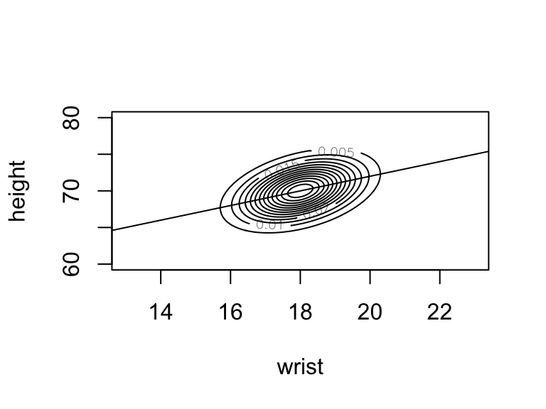
What is the expected value of height \(Y\) when \(X=x\), \(E(Y|X=x)\)? Rearrange this expected value so that it’s in the form \(aX + b\).
Sketch this expected value. Specifically, on your paper, superimpose the expected value line \(E(Y|X=x) = aX + b\) on the contour plot shown above.
IMPORTANT CONNECTION:
If you’ve taken STAT 155, you should recognize that this is a linear regression line. Though you didn’t dive into theory in STAT 155, the assumption behind the models you explored in that class is that \(Y|(X=x) \sim N(ax+b, \sigma^2)\). The coefficients \(a,b\) of this theoretical relationship are estimated from observed data.
Solution
\[\begin{split} Y|(X=x) & \sim N\left(70 + \frac{2.5}{1}*0.4*(x - 18), (1 - 0.4^2) 2.5^2 \right) \\ & \sim N(70 + (x-18), 5.25) \\ & \sim N(x + 52, 2.29^2) \\ \end{split}\]
x + 52
- .
- State the conditional model of height \(Y\) given the information that \(X=x\). Simplify parameters as much as possible.
- General observations
For the remainder of the exercises, abandon the context of wrists and heights to consider general properties of the bivariate Normal model. In our general formulations above, we defined the conditional Normal model of \(Y\) given \(X = x\) by \[Y|(X=x) \sim N \left(\mu_Y + \frac{\sigma_Y}{\sigma_X} \rho (x-\mu_X), \; (1-\rho^2)\sigma_Y^2\right)\]Explain the impact that \(\rho\) has on the conditional variance \(Var(Y|(X=x))\). Why does this make intuitive sense?
Rewrite \(E(Y|(X=x))\) in the form \(E(Y|(X=x)) = ax + b\).
Solution
As \(\rho \to 1\) or \(\rho \to -1\) (ie. the stronger the correlation between \(X\) and \(Y\)), the conditional variability in \(Y\) goes to 0: \[(1-\rho^2)\sigma^2_Y \to 0\] Intuitively, this makes sense. If there’s a strong relationship between \(X\) and \(Y\), then if we know \(X\), this provides precise information about \(Y\) (with little variability).
- .
\[\left(\frac{\sigma_Y}{\sigma_X}\rho\right) x + \left(\mu_Y - \frac{\sigma_Y}{\sigma_X}\rho \mu_X\right)\]
Independence vs Correlation
In the above exercises, wrist circumference and height were correlated (\(\rho \ne 0\)). In the exercises below, let \(X\) and \(Y\) be two generic RVs (not wrist circumference and height specifically). Further, recall that the correlation between two RVs \(X\) and \(Y\) is calculated by\[\rho = \frac{E((X-E(X))(Y - E(Y)))}{\sqrt{Var(X)Var(Y)}}\;.\]
Let \(Y = aX + b\) with \(a>0\), ie. \(Y\) is a linear transformation of \(X\). For example \(Y\) might be the conversion of a measurement \(X\) from inches to centimeters. Calculate the correlation between \(X\) and \(Y\).
Suppose \(X\) and \(Y\) are independent. Prove that \(X\) and \(Y\) must be uncorrelated (\(\rho=0\)). HINT: You can use the fact that if \(X\) and \(Y\) are independent, then \[\begin{split} E((X-E(X))(Y-E(Y))) & = \int\int (x-E(X))(y-E(Y))f_{X,Y}(x,y)dxdy = \\ & = \int\int (x-E(X))(y-E(Y))f_{X,Y}(x,y)dxdy \\ & = \int\int (x-E(X))(y-E(Y))f_{X}(x)f_{Y}(y)dxdy \;\; \text{ (by independence)} \\ & = \int (x-E(X)) f_X(x)dx \int (y-E(Y))f_{Y}(y)dy \\ & = E(X-E(X))E(Y-E(Y)) \\ \end{split} \]
In part b you showed that independence between two RVs guarantees that they’re uncorrelated. The opposite is not true. Consider the following example. Suppose \(X \sim N(0,1)\) and \(Y = X^2\) with \(E(X) = 0\). Thus \(X\) and \(Y\) are clearly dependent. However, show that they are uncorrelated.
HINT: \(E(XY) = E(X^3)\).
EXPLANATION
Correlation measures the strength and direction of a linear relationship. Though \(Y=X^2\) is perfectly determined by thus dependent upon \(X\), the relationship between the 2 is non-linear. Thus their correlation is 0. The following simulation provides intuition:x <- rnorm(10000) y <- x^2 # Estimate the correlation: note it's essentially 0 cor(x,y) ## [1] -0.00949124 # Plot the data: note the dependence! sim_data <- data.frame(x, y) ggplot(sim_data, aes(x=x, y=y)) + geom_point()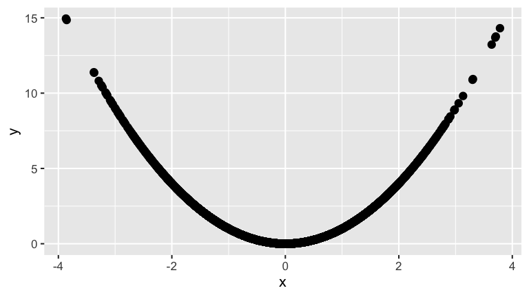
Solution
.
\[\begin{split} \rho & = \frac{E((X-E(X))(Y - E(Y)))}{\sqrt{Var(X)Var(Y)}} \\ & = \frac{E((X-E(X))((aX + b) - E(aX + b)))}{\sqrt{Var(X)Var(aX + b)}} \\ & = \frac{E((X-E(X))((aX + b) - (aE(X) + b)))}{\sqrt{Var(X)* a^2Var(X)}} \\ & = \frac{E((X-E(X)) * a(X - E(X)))}{\sqrt{a^2*(Var(X))^2}} \\ & = \frac{aE((X-E(X))^2)}{aVar(X)} \\ & = \frac{aVar(X)}{aVar(X)} \\ & = 1 \\ \end{split}\].
\[\begin{split} \rho & = \frac{E((X-E(X))(Y - E(Y)))}{\sqrt{Var(X)Var(Y)}} \\ & = \frac{E(X-E(X))E(Y - E(Y))}{\sqrt{Var(X)Var(Y)}} \\ & = \frac{(E(X)-E(X))(E(Y) - E(Y))}{\sqrt{Var(X)Var(Y)}} \\ & = 0 \\ \end{split}\]For \(X \sim N(0,1^2)\),
\[\begin{split} E(X) & = 0 \\ Var(X) & = E(X^2) - [E(X)]^2 = 1 \\ E(X^2) & = Var(X) - [E(X)]^2 = 1 - 0 = 1 \\ E(X^3) & = E((X - E(X))^3) = 0 \;\; \text{(since the Normal is symmetric)} \\ \end{split}\] It follows that \[\begin{split} \rho & = \frac{E((X-E(X))(Y - E(Y)))}{\sqrt{Var(X)Var(Y)}} \\ & = \frac{E((X-E(X))(X^2 - E(X^2)))}{\sqrt{Var(X)Var(X^2)}} \\ & = \frac{E((X-0)(X^2 - 1))}{\sqrt{Var(X)Var(X^2)}} \\ & = \frac{E(X^3 - X)}{\sqrt{Var(X)Var(X^2)}} \\ & = \frac{E(X^3) - E(X)}{\sqrt{Var(X)Var(X^2)}} \\ & = \frac{0 - 0}{\sqrt{Var(X)Var(X^2)}} \\ & = 0 \\ \end{split}\]
- EXTRA (if you have time)
Assume \(X, Y\) are jointly Normal:
\[\left(\begin{array}{c} X \\ Y \end{array}\right) \sim N \left(\left(\begin{array}{c} \mu_X \\ \mu_Y \end{array}\right), \; \left(\begin{array}{cc} \sigma^2_X & \rho \sigma_X \sigma_Y\\ \rho \sigma_X \sigma_Y & \sigma^2_Y \end{array}\right) \right) \;\; \] and prove that \[ Y|(X=x) \sim N \left(\mu_Y + \frac{\sigma_Y}{\sigma_X} \rho (x-\mu_X), \; (1-\rho^2)\sigma_Y^2\right) \]