17 Moments
Goal
Before moving on to multivariate probability models, we’ll examine one more feature of univariate probability models: moments.
READING
For more on this topic, read B & H Chapter 6.
17.1 Discussion
RECALL:
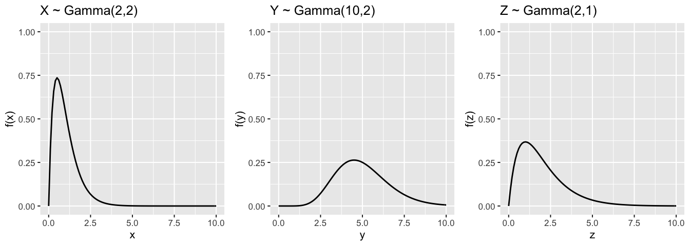
The Gamma(\(a,\lambda\)) model can be used to model the waiting time for \(a\) events where events occur at a rate of \(\lambda\):
MOTIVATING EXAMPLE
Let
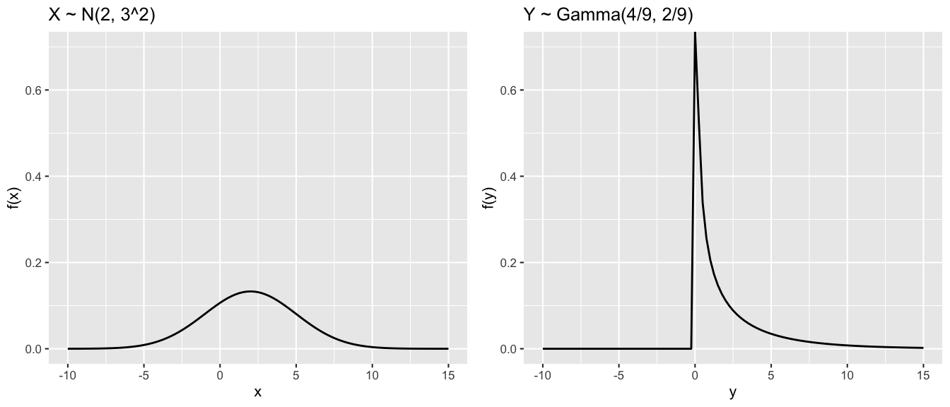
\[X \sim N(2, 3^2) \;\; \text{ and } \;\; Y \sim \text{Gamma}(4/9, 2/9)\]
Then using the general properties of the Normal and Gamma models,
| Model | \(E(X)\) | \(Var(X)\) |
|---|---|---|
| \(X \sim N(\mu,\sigma^2)\) | \(\mu\) | \(\sigma^2\) |
| \(X \sim \text{Gamma}(a, \lambda)\) | \(a / \lambda\) | \(a / \lambda^2\) |
We can show that \(X\) and \(Y\) have the same mean and variance:
\[\begin{array}{rlcrl} E(X) & = 2 & \hspace{1in} & E(Y) & = \frac{4/9}{2/9} = 2 \\ Var(X) & = 3^2 = 9 & & Var(Y) & = \frac{4/9}{(2/9)^2} = 9 \\ \end{array}\]
Question:
Do \(X\) and \(Y\) have the same model? That is, are the \(N(2, 3^2)\) and \(Gamma(4/9,2/9)\) models equivalent?
Answer: NO!
\(E()\) and \(Var()\) provide measures of trend and deviation from trend. But they don’t capture every important feature. \(X\) and \(Y\) are otherwise very different:
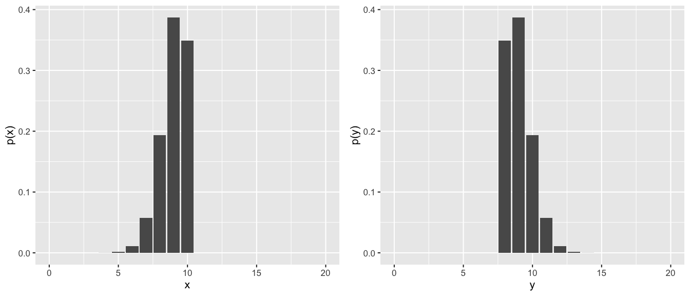
For another example, the discrete RVs corresponding to the PMFs below both have \(E(X)=9\) and \(Var(X)=0.9\):
WHAT’S THE POINT?
\(E(X)\) and \(Var(X)\) capture two important but relatively small features of the probability model for \(X\). We need to study other moments of \(X\).
Moments
Define notation: \[\begin{split} \mu & := E(X) \\ \sigma^2 & := Var(X) \\ \sigma & := SD(X) \\ \end{split}\]
Define “moments”:
\[\begin{split} E(X^k) & = k\text{th moment of } X \\ E[(X-\mu)^k] & = k\text{th central moment of } X \\ E\left[\left(\frac{X-\mu}{\sigma}\right)^k\right] & = k\text{th standardized moment of } X \\ \end{split}\]
Moments capture key features of a probability model. For example, \[\begin{split} \text{Center}: & \; \; \; E(X) = 1\text{st moment} \\ \text{Spread}: & \; \; \;Var(X) = E[(X-\mu)^2] = 2\text{nd central moment}\\ \text{Skew}: & \; \; \; Skew(X) = E\left[\left(\frac{X-\mu}{\sigma}\right)^3\right] = 3\text{rd standardized moment}\\ \end{split}\]
NOTE: If \(X\) has a symmetric pdf/pmf, then \(Skew(X)=0\).
EXAMPLE 1
For \(Z \sim Gamma(a,\lambda)\) with pdf \(f_Z(z) = \frac{\lambda^a}{\Gamma(a)}z^{a-1}e^{-\lambda z}\) for \(z > 0\):
\[\begin{split} \mu & = E(Z) = \frac{a}{\lambda} \\ \sigma^2 & = Var(Z) = \frac{a}{\lambda^2} \\ Skew(Z) & = E\left[\left(\frac{Z-\mu}{\sigma}\right)^3\right] = \frac{2}{\sqrt{a}} \\ \end{split}\]
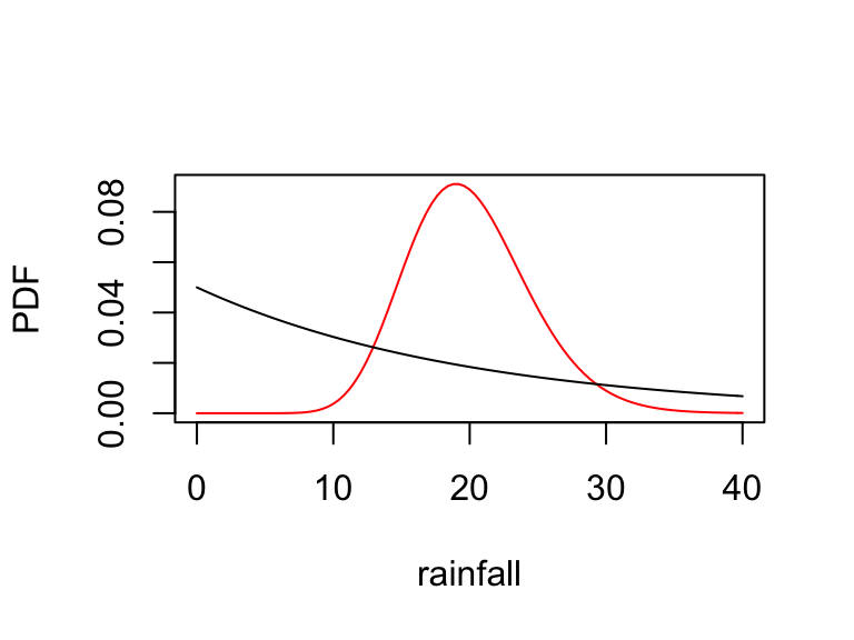
For example, Gammas can be used for more than modeling waiting times – meteorologists have found that country-level rainfall can be modeled by a Gamma model. Suppose
\(X \sim Gamma(1,0.05)\): rainfall in country A (in inches)
\(Y \sim Gamma(20,1)\): rainfall in country B (in inches)
The PDFs of \(X\) (black) and \(Y\) (red) are plotted below:
Thus for rainfall measurements \(X\) and \(Y\):
\[\begin{array}{rlcrl} E(X) & = \frac{1}{0.05} = 20 \text{ inches} & \hspace{1in} & E(Y) & = \frac{20}{1} = 20 \text{ inches} \\ Var(X) & = \frac{1}{0.05^2} = 400 \text{ inches}^2 && Var(Y) & = \frac{20}{1^2} = 20 \text{ inches}^2 \\ Skew(X) & = \frac{2}{\sqrt{1}} = 2 \text{ inches}^3 && Skew(Y) & = \frac{2}{\sqrt{20}} \approx 0.45 \text{ inches}^3 \\ \end{array}\]
According to the pictures and math, which of \(X\) and \(Y\) is less skewed?
Show that a Gamma(\(a,\lambda\)) RV has \(Skew(Z) = E\left[\left(\frac{Z-\mu}{\sigma}\right)^3\right] = \frac{2}{\sqrt{a}}\).
Just kidding.
A SNAG
Calculating moments is important but can require tedious summation or integration. For example, \[ E(X^k) = \int_{-\infty}^\infty x^k f_X(x) dx \;\;\; \text{ for continuous } X \; . \] Instead of calculating moments individually, we can use moment generating functions (MGF).
Moment Generating Functions (MGFs)
The moment generating function (mgf) of RV \(X\) is \[M_X(t) = E(e^{tX}) = \begin{cases} \sum_{\text{all } x}e^{tx}p_X(x) & X \text{ discrete } \\ \int_{-\infty}^\infty e^{tx} f_X(x)dx & X \text{ continuous} \\ \end{cases}\]
The mgf has many applications:
identifying models
proving the Central Limit Theorem! (we haven’t covered this yet, but it will be important later on)
calculating moments
\[\begin{split} E(X) & = \text{ first "moment" of $X$ } = M_X^{(1)}(0) \\ E(X^2) & = \text{ second "moment" of $X$ } = M_X^{(2)}(0) \\ E(X^k) & = \text{ $k$th "moment" of $X$ } = M_X^{(k)}(0) \\ \end{split}\]Specifically, to calculate \(M_X^{(k)}(0)\): Take the \(k\)th derivative of \(M_X(t)\) with respect to \(t\). Then plug in 0 for \(t\).
EXAMPLE 2: Exponential MGF
Let \(X \sim \text{Exp}(\lambda)\) with PDF \[f_X(x) = \lambda e^{-\lambda x} \;\; \text{ x > 0}\]
We could show the “old” way that \[\begin{split} E(X) & = \int_0^\infty x \cdot \lambda e^{-\lambda x} dx = \frac{1}{\lambda} \\ E(X^2) & = \int_0^\infty x^2 \cdot \lambda e^{-\lambda x} dx = \frac{2}{\lambda^2} \\ Var(X) & = E(X^2) - [E(X)]^2 = \frac{2}{\lambda^2} - \left(\frac{1}{\lambda}\right)^2 = \frac{1}{\lambda^2} \\ \end{split}\]
- Show that for \(t < \lambda\), the mgf of \(X\) is \[M_X(t) = E(e^{tX}) = \frac{\lambda}{\lambda - t}\]
- Calculate \(E(X)\) and \(E(X^2)\) (hence \(Var(X)\)) using the mgf. HINTS:
\[\begin{split} \frac{d}{dt} \frac{\lambda}{\lambda - t} & = \frac{\lambda}{(\lambda - t)^{2}} \\ \frac{d}{dt}\frac{\lambda}{(\lambda - t)^{2}}& = \frac{2\lambda}{(\lambda - t)^{3}} \\ \end{split}\]
17.2 Exercises
17.2.1 Part 1: MGFs for common models
Just like PDFs/PMFs/CDFs, MGFs are unique! If 2 variables have the same MGF, they have the same model. The following table summarizes the MGFs for some of our favorite models:
| model | \(E(X)\) | \(Var(X)\) | \(M_X(t)\) |
|---|---|---|---|
| Bern(\(n,p\)) | \(p\) | \(p(1-p)\) | \(1 - p + pe^t\) |
| Bin(\(n,p\)) | \(np\) | \(np(1-p)\) | \((1 - p + pe^t)^n\) |
| Geo(\(p\)) | \(\frac{1}{p}\) | \(\frac{1-p}{p^2}\) | \(\frac{pe^t}{1 - (1-p)e^t}\) |
| Exp(\(\lambda\)) | \(\frac{1}{\lambda}\) | \(\frac{1}{\lambda^2}\) | \(\frac{\lambda}{\lambda - t}\) for \(t < \lambda\) |
| Gamma(\(a,\lambda\)) | \(\frac{a}{\lambda}\) | \(\frac{a}{\lambda^2}\) | \(\left(\frac{\lambda}{\lambda-t}\right)^a\) for \(t < \lambda\) |
Bernoulli: Derive & apply the MGF
Let \(X \sim Bern(p)\) (equivalently, \(X \sim Bin(1,p)\)). That is, \(X\) is the number of successes in 1 trial where probability of success is \(p\). Then \(X\) has pmf \[p_X(x) = p^x(1-p)^{1-x} \;\; \text{ for } x \in\{0,1\}\]Prove that \(X\) has mgf \(M_X(t) = E(e^{tX}) = 1 - p + pe^t\).
Use the mgf to show that \(E(X)=p\).
Use the mgf to calculate \(E(X^2) = p\).
Combine a and b to prove that \(Var(X)=p(1-p)\).
Use MGFs to name that model
If you learned that RV \(X\) has mgf \(M_X(t) = \frac{1}{1-t}\), then by the table above, you’d know that \(X \sim Exp(1)\). That is, if we plug in \(\lambda=1\) into \(M_X(t) = \frac{\lambda}{\lambda - t}\), we get \(M_X(t) = \frac{1}{1-t}\). Similarly, use the MGFs given below to identify the model of the corresponding RV \(X\).\(M_X(t) = \frac{3}{3-2t}\)
\(M_X(t) = (0.25 + 0.75e^{t})^{22}\)
\(M_X(t) = \left(\frac{3}{3-t}\right)^2\)
\(M_X(t) = \frac{0.9e^t}{1-0.1e^t}\)
17.2.2 Part 2: MGF’s for linear transformations
Let RV \(X\) have mgf \(M_X(t)\). Further, let \(Y\) be a linear transformation of \(X\), \[Y=aX+b\] You’ll show below that
\[M_Y(t) = E(e^{tY}) = e^{bt}M_X(at)\]
Let’s apply this before proving it!
MGFs for identifying models of transformed RVs
MGFs are really handy in identifying models. For example, let \(X\) be the waiting time (in minutes) in the first aisle of a grocery store and suppose that \(X \sim Exp(0.01)\). Further, let \(Y\) be the waiting time in the second aisle and suppose \(Y = 2X\).Before doing any math, check your intuition. How can we interpret \(Y\) and what model do you think it should have?
Write out the mgf of \(X\), \(M_X(t)\).
Recall that if \(Y=aX+b\), then \(M_Y(t) = E(e^{tY}) = e^{bt}M_X(at)\). Use this to derive the mgf of \(Y\), \(M_Y(t)\).
Use \(M_Y(t)\) to identify the model of \(Y\) - give the name of this model as well as the values of any defining parameters. Does this match your intuition? NOTE: You’ll have to rearrange \(M_Y(t)\).
Extra Practice (to do after class, not now)
In part d you used the MGF trick to identify the model of \(Y\). As an alternative solution, calculate the pdf of \(Y\) and show that this is consistent with the model of \(Y\) you derived above using the MGF. NOTE: There are a few intermediate steps that are left out. Try to fill these in on your own.
CHALLENGE: MGFs for linear transformations
Let RV \(X\) have mgf \(M_X(t)\). Further, let \(Y\) be a linear transformation of \(X\), \[Y=aX+b\]Prove that the mgf of \(Y\) can be defined by the mgf of \(X\): \[M_Y(t) = E(e^{tY}) = e^{bt}M_X(at)\] Try this on your own before looking at the hints below.
HINT 1:
\(e^{tY} = e^{t(aX+b)}\)
HINT 2:
\(e^{tY} = e^{t(aX+b)} = e^{(at)X + bt}\)
HINT 3:
\(e^{tY} = e^{t(aX+b)} = e^{(at)X + bt} = e^{(at)X}e^{bt}\)
HINT 4:
\(e^{bt}\) is a constant
Calculate \(E(Y)\) from \(M_Y(t)\). Again, you should see that \(E(Y) = aE(X)+b\).
HINT 1: By the product rule,
\(\frac{d}{dt}M_Y(t) = \frac{d}{dt}\left[e^{bt}M_X(at)\right] = \frac{d}{dt}\left[e^{bt}\right]\cdot M_X(at) + e^{bt}\cdot \frac{d}{dt}\left[M_X(at)\right]\)
HINT 2: By the chain rule,
\(\frac{d}{dt}\left[e^{bt}\right] = be^{bt}\)
\(\frac{d}{dt}\left[M_X(at)\right] = a\cdot M_X'(at)\)
17.2.3 Part 3: Proof
- Proof that the MGF calculates moments
We’ve been using the fact that we can calculate moments using MGFs: \(E(X^k)=M_X^{(k)}(0)\). Prove that this is true. To this end, you can use the fact that \(e^{tX}\) has the following series expansion: \[e^{tX} = \sum_{i=0}^\infty \frac{(tX)^i}{i!} = 1 + tX + \frac{t^2X^2}{2!} + \frac{t^3X^3}{3!} + \cdots \]