10 Properties of RVs: Expected Value & Variance

READING:

For more on this topic, read B & H Chapter 4.1 & 4.6.

10.1 Discussion

OVERARCHING GOAL OF UNIT 2
Explore univariate probability models.

BIG QUESTION 1: What model is appropriate for any given random variable?

BIG QUESTION 2: What are the features of this model? How might data generated from this model behave in the long run?

Measuring central tendency: Expected Value of $X$
$E(X)$ measures the trend in, or long-run average of, $X$. It’s calculated as a weighted average of all possible values of $X$ (ie. each possible $x$ is weighted by its corresponding PMF $p_X(x)$ or PDF $f_X(x)$) \[\begin{split} \text{discrete $X$: } & \;\;\; E(X) = \sum_{\text{all } x} x \; p_X(x) \\ \text{continuous $X$: } & \;\;\; E(X) = \int_{\text{all } x} x \; f_X(x)dx \\ \end{split}\]

Similarly, let $g(X)$ be some function of RV $X$. Then \[\begin{split} \text{discrete $X$: } & \;\;\; E(g(X)) = \sum_{\text{all } x} g(x) \; p_X(x) \\ \text{continuous $X$: } & \;\;\; E(g(X)) = \int_{\text{all } x} g(x) \; f_X(x)dx \\ \end{split}\]

NOTE: $E(X)$ is reflected in the sample mean of a sample of data $(X_1,X_2,...,X_n)$, $\overline{x} = \frac{1}{n}\sum_{i=1}^n x_i$.

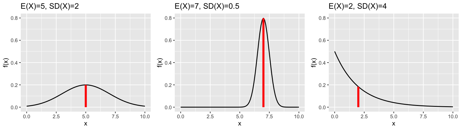
Measuring spread: Variance & Standard Deviation of $X$

$Var(X)$ measures the typical squared deviation from the trend, or long-run variance of, $X$. $SD(X)$ measures the typical deviation from the trend, or long-run standard deviation of, $X$. \[\begin{split} Var(X) & = E((X - E(X))^2) = \begin{cases} \sum_{\text{all } x} (x - E(X))^2 \; p_X(x) & \;\; X \text{ discrete} \\ \int_{\text{all } x} (x - E(X))^2 \; f_X(x)dx & \;\; X \text{ continuous} \\ \end{cases} \\ Var(X) & = E(X^2) - \left[E(X)\right]^2 \;\;\;\;\; \text{(typically easier to calculate!)}\\ SD(X) & = \sqrt{Var(X)} \\ \end{split}\]

NOTE: $Var(X)$ is reflected in the sample variance of a sample of data $(X_1,X_2,...,X_n)$, $\overline{x} = \frac{1}{n-1}\sum_{i=1}^n (x_i - \overline{x})^2$.

EXAMPLE 1

Let $X$ be the measurement error of a weighing device (in pounds) used by a certain company.

$x$	-1	0	1	2	Total
$p_X(x)$	0.4	0.3	0.2	0.1	1

Calculate $E(X)$, the typical measurement error.
Calculate $E(X^2)$, tye typical squared measurement error.
Calculate $Var(X)$, the variance in the weighing errors, two ways: \[\begin{split} Var(X) & = E((X - E(X))^2) = \sum_{\text{all } x} (x - E(X))^2 p_X(x) \\ Var(X) & = E(X^2) - \left[E(X)\right]^2 \\ \end{split}\]

EXAMPLE 2

Consider a generic discrete RV $X$. Show that \[Var(X) = E((X - E(X))^2) = E(X^2) - \left[E(X)\right]^2\]

HINT: Note that $E(X)$ is a constant.

The Uniform model
Suppose random variable $X$ is equally / uniformly distributed across the interval $[a, b]$. In notation, \[X \sim Unif(a, b)\] with pdf \[f_X(x) = \frac{1}{b-a} \;\; \text{ for } x \in [a,b]\] Thus the behavior of $X$ depends upon parameters $a$ and $b$. Prove that \[\begin{split} E(X) & = \frac{1}{2}(a + b) \\ Var(X) & = E(X^2) - [E(X)]^2 = \frac{1}{12}(b - a)^2\\ \end{split}\] NOTE: The features of the following Uniforms will help confirm your work.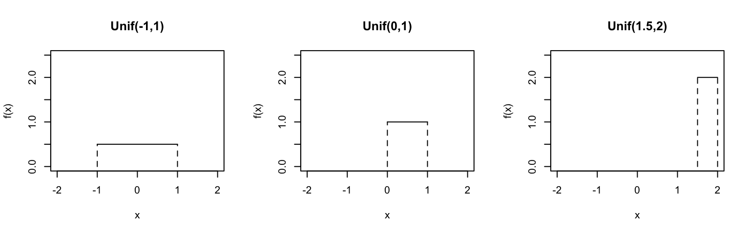

Model $E(X)$ $Var(X)$ $SD(X)$

Unif(-1,1) 0 0.333 0.577

Unif(0,1) 0.50 0.083 0.289

Unif(1.5,2) 1.75 0.021 0.144

Model	\(E(X)\)	\(Var(X)\)	\(SD(X)\)
Unif(-1,1)	0	0.333	0.577
Unif(0,1)	0.50	0.083	0.289
Unif(1.5,2)	1.75	0.021	0.144

The Binomial model: gut check
Let $X \sim Bin(n,p)$. Thus the behavior of $X$ depends upon parameters $n$ and $p$. Use your gut to answer the following questions.
1. Let $X$ be the number of Heads in 100 flips ($X \sim Bin(100, 0.5)$). What’s $E(X)$, ie. how many Heads would you expect?
2. Let $X$ be the number of 1s in 24 dice rolls ($X \sim Bin(24, 1/6)$). What’s $E(X)$, ie. how many 1s would you expect?
3. Generalize it: Let $X \sim Bin(n,p)$. What’s a general formula for $E(X)$? NOTE: this formula should depend upon $n$ and $p$.

The Binomial model
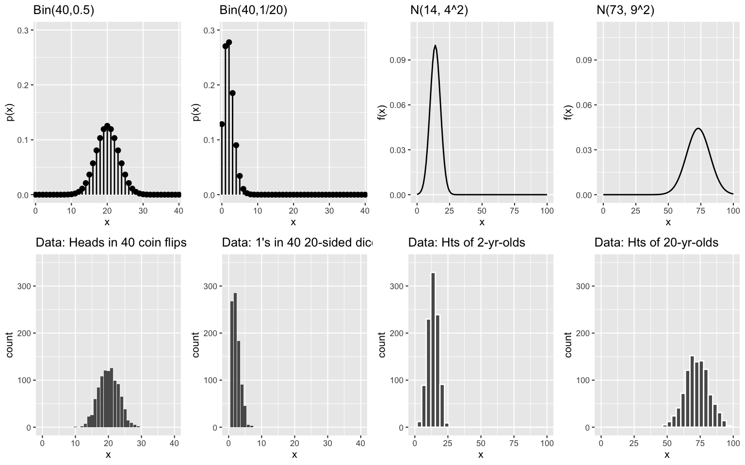
Let $X \sim Bin(n,p)$ with PMF \[p_X(x) = \left(\begin{array}{c} n \\ x \end{array} \right) p^x (1-p)^{n-x} \; \text{ for } \in x \in \{0,1,...,,n\}\] Then \[\begin{split} E(X) & = \sum_{\text{all } x} x p_X(x) = np \\ Var(X) & = E\left[(X - E(X))^2\right] = E(X^2) - \left[E(X)\right]^2 = np(1-p) \\ \end{split}\]
1. Calculate $E(X)$ and $Var(X)$ for each Binomial model below:
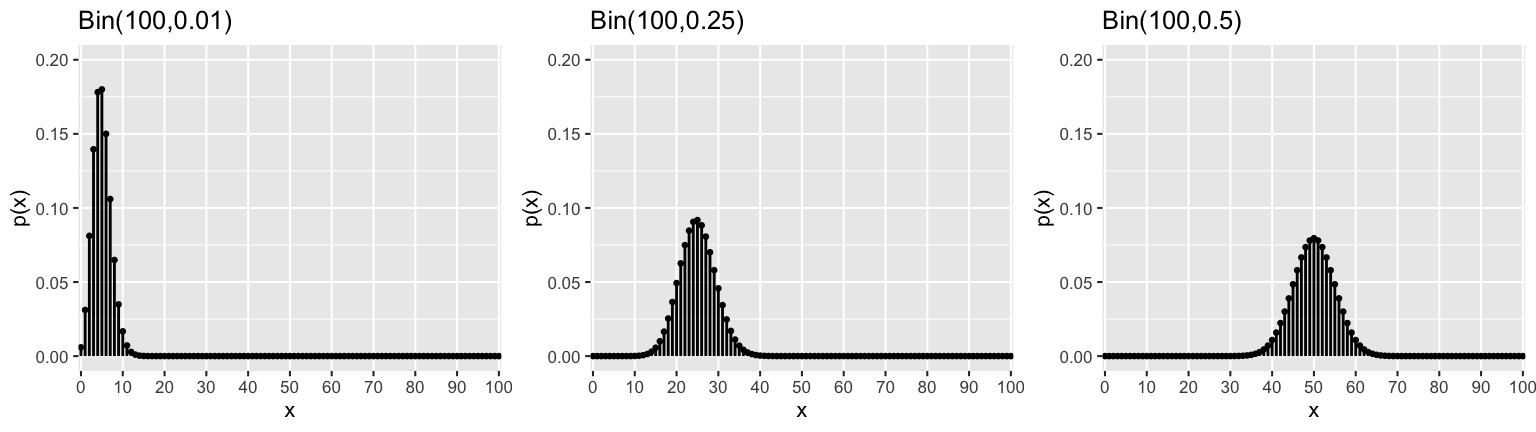
2. For what value of $p$ is $Var(X)$ maximized? Why does this make intuitive sense?
3. CHALLENGE: prove that $E(X) = np$ and $Var(X) = np(1-p)$. This is quite tricky and will be easier after we get some practice with other RVs.

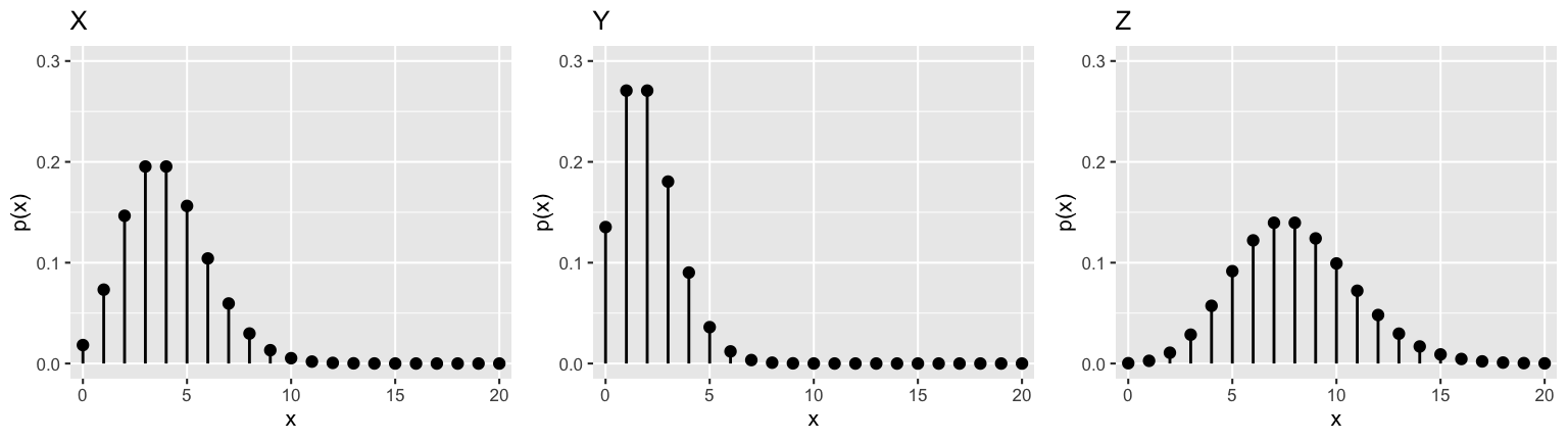
The Poisson model
Let $X \sim Pois(\lambda)$ with PMF \[p_X(x) = \frac{\lambda^x e^{-\lambda}}{x!} \; \text{ for } \in x \in \{0,1,2,...\}\] Then the Poisson expected value and variance are both equal to $\lambda$: \[\begin{split} E(X) & = \sum_{\text{all } x} x p_X(x) = \lambda \\ Var(X) & = E\left[(X - E(X))^2\right] = E(X^2) - \left[E(X)\right]^2 = \lambda \\ \end{split}\]
1. On average, calls come into a call center at a rate of 4 per minute. Let $X$ number of calls in 1 minute. Thus $X \sim Pois(4)$. Calculate $E(X)$ and $SD(X)$, the expected number of calls and standard deviation of calls per minute.
2. Let $Y$ be the number of calls in 30 seconds. Thus $Y$ is Poisson with rate $\lambda$. Identify $\lambda$ and calculate $E(Y)$ and $SD(Y)$.
3. Let $Z$ be the number of calls in 2 minutes. Thus $Z$ is Poisson with some rate $\lambda$. Identify $\lambda$ and calculate $E(Z)$ and $SD(Z)$.

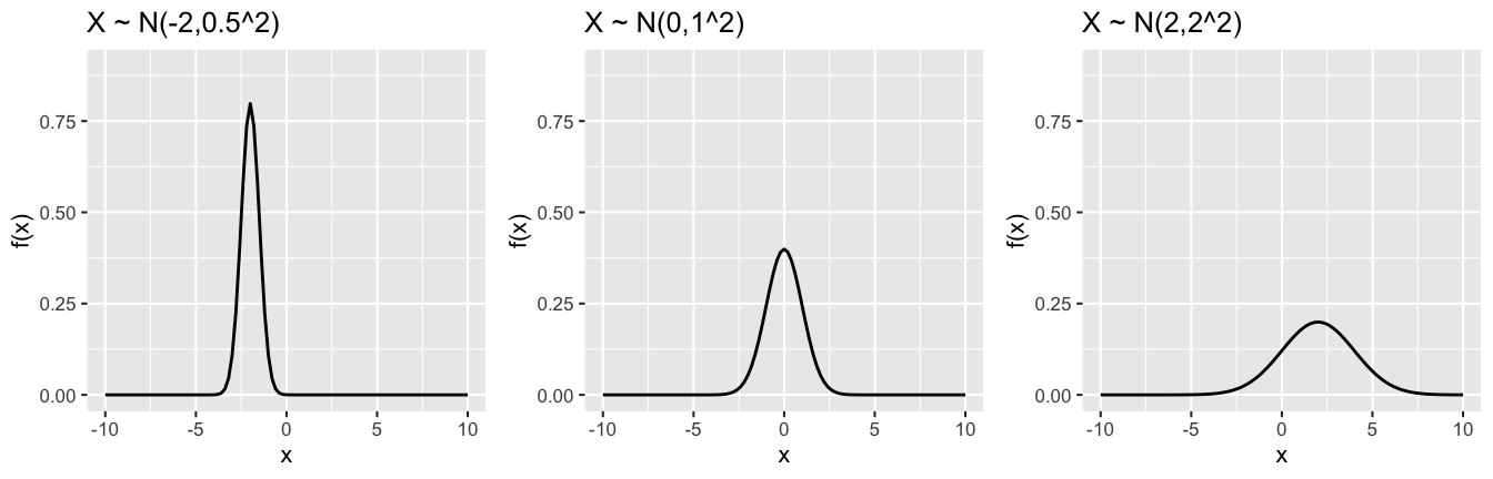
The Normal model
Let $X \sim N(\mu, \sigma^2)$. Then $E(X) = \mu$ and $Var(X) = \sigma^2$.